

Antibody-antigen modelling tutorial using a local version of HADDOCK3
This tutorial consists of the following sections:
- Introduction
- HADDOCK general concepts
- A brief introduction to HADDOCK3
- Software and data setup
- Preparing PDB files for docking
- Defining restraints for docking
- Setting up and running the docking with HADDOCK3
- HADDOCK3 workflow definition
- Running HADDOCK3
- Execution of HADDOCK3 on the computers of the BioExcel 2026 summerschool
- Execution of HADDOCK3 on DISCOVERER (BioExcel Sofia May 2025 workshop)
- Execution of HADDOCK3 on the TRUBA resources (EuroCC Istanbul April 2024 workshop)
- Execution of HADDOCK3 on Fugaku (ASM 2026 HPC/AI school, Kobe Japan)
- Execution of HADDOCK3 on ADD Ljubljana (BioExcel Adriatic edition 2026, Ljubljana, Slovenia)
- Learn more about the various execution modes of haddock3
- Analysis of docking results
- Conclusions
- BONUS 1: Dissecting the interface energetics: what is the impact of a single mutation?
- BONUS 2: Does the antibody bind to a known interface of interleukin? ARCTIC-3D analysis
- BONUS 3: How good are AI-based models of antibody for docking?
- BONUS 4: Ensemble docking using a combination of exprimental and AI-predicted antibody structures
- BONUS 5: Antibody-antigen complex structure prediction from sequence using AlphaFold2
- BONUS 6: Running a scoring scenario
- Congratulations! 🎉
Introduction
This tutorial demonstrates the use of the new modular HADDOCK3 version for predicting the structure of an antibody-antigen complex using knowledge of the hypervariable loops on the antibody (i.e., the most basic knowledge) and epitope information identified from NMR experiments for the antigen to guide the docking.
The associated data and presented results in this tutorial were obtained with HADDOCK3 version 2026.5.0 running on Mac with arm2 processors.
The command line version of this tutorial was recorded at the BioExcel Sofia Workshop in May 2025:
- View recorded command line tutorial
And the Jupyter notebook version was recorded at the ASEAN ASM HPC school in Kope, Japan, in January 2026:
- View recorded Jupyter notebook HADDOCK3 practical Part I (46 min.)
- View recorded Jupyter notebook HADDOCK3 practical Part II (46 min.)
An antibody is a large protein that generally works by attaching itself to an antigen,
which is a unique site of the pathogen. The binding harnesses the immune system to directly
attack and destroy the pathogen. Antibodies can be highly specific while showing low immunogenicity (i.e. the ability to provoke an immune response),
which is achieved by their unique structure. The fragment crystallizable region (Fc region)
activates the immune response and is species-specific, i.e. the human Fc region should not
induce an immune response in humans. The fragment antigen-binding region (Fab region)
needs to be highly variable to be able to bind to antigens of various nature (high specificity).
In this tutorial, we will concentrate on the terminal variable domain (Fv) of the Fab region.
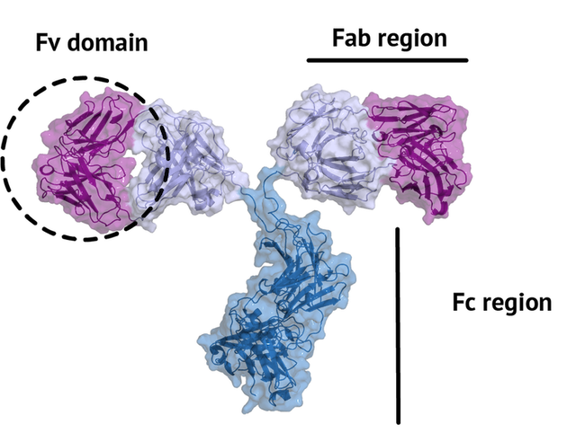
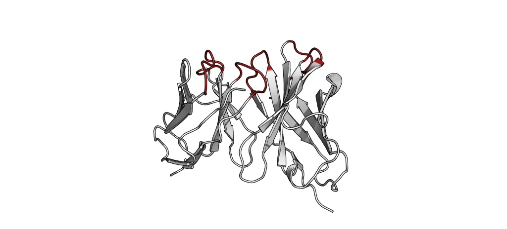
The small part of the Fab region that binds the antigen is called paratope. The part of the antigen that binds to an antibody is called epitope. The paratope consists of six highly flexible loops, known as complementarity-determining regions (CDRs) or hypervariable loops whose sequence and conformation are altered to bind to different antigens. CDRs are shown in red in the figure below:
In this tutorial we will be working with Interleukin-1β (IL-1β) (PDB code 4I1B) as an antigen and its highly specific monoclonal antibody gevokizumab (PDB code 4G6K) (PDB code of the complex 4G6M).
Throughout the tutorial, colored text will be used to refer to questions or instructions, and/or PyMOL commands.
This is a question prompt: try answering it! This an instruction prompt: follow it! This is a PyMOL prompt: write this in the PyMOL command line prompt! This is a Linux prompt: insert the commands in the terminal!
HADDOCK general concepts
HADDOCK (see https://www.bonvinlab.org/software/haddock2.4) is a collection of python scripts derived from ARIA (https://aria.pasteur.fr) that harness the power of CNS (Crystallography and NMR System – https://cns-online.org) for structure calculation of molecular complexes. What distinguishes HADDOCK from other docking software is its ability, inherited from CNS, to incorporate experimental data as restraints and use these to guide the docking process alongside traditional energetics and shape complementarity. Moreover, the intimate coupling with CNS endows HADDOCK with the ability to actually produce models of sufficient quality to be archived in the Protein Data Bank.
A central aspect of HADDOCK is the definition of Ambiguous Interaction Restraints or AIRs. These allow the translation of raw data such as NMR chemical shift perturbation or mutagenesis experiments into distance restraints that are incorporated into the energy function used in the calculations. AIRs are defined through a list of residues that fall under two categories: active and passive. Generally, active residues are those of central importance for the interaction, such as residues whose knockouts abolish the interaction or those where the chemical shift perturbation is higher. Throughout the simulation, these active residues are restrained to be part of the interface, if possible, otherwise incurring a scoring penalty. Passive residues are those that contribute to the interaction but are deemed of less importance. If such a residue does not belong in the interface there is no scoring penalty. Hence, a careful selection of which residues are active and which are passive is critical for the success of the docking.
A brief introduction to HADDOCK3
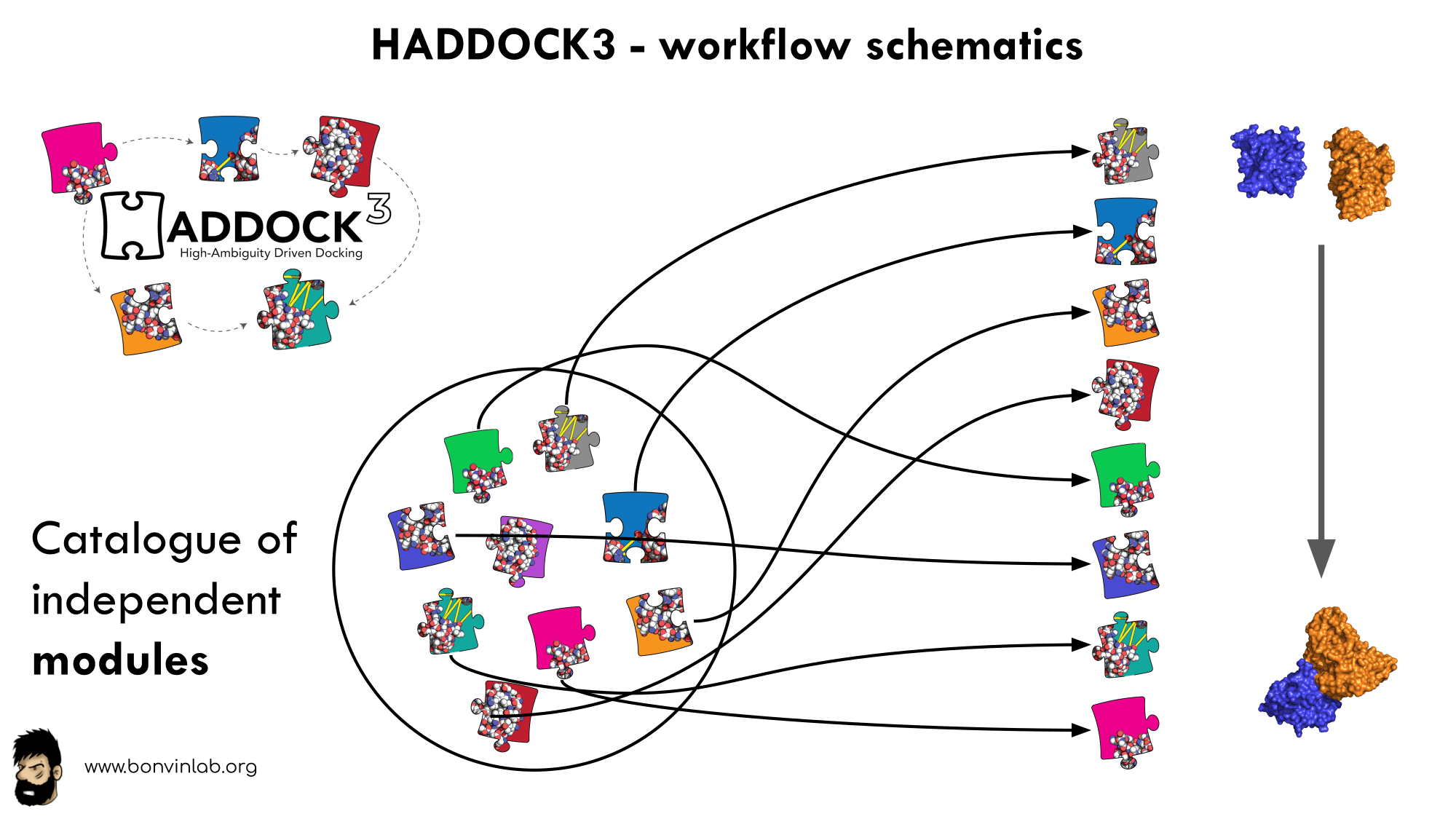
HADDOCK3 is the next generation integrative modelling software in the long-lasting HADDOCK project. It represents a complete rethinking and rewriting of the HADDOCK2.X series, implementing a new way to interact with HADDOCK and offering new features to users who can now define custom workflows.
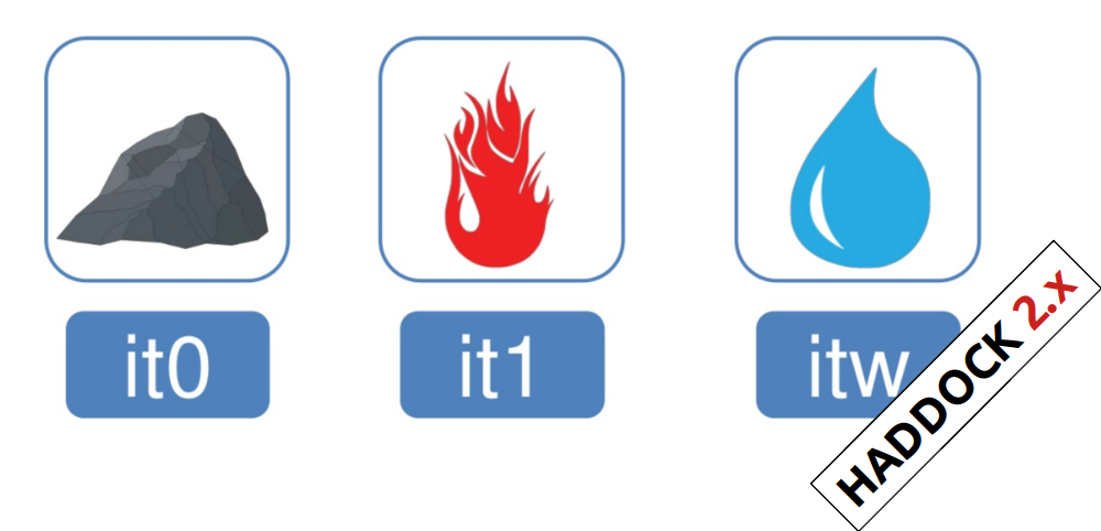
In the previous HADDOCK2.x versions, users had access to a highly
parameterisable yet rigid simulation pipeline composed of three steps:
rigid-body docking (it0), semi-flexible refinement (it1), and final refinement (itw).
In HADDOCK3, users have the freedom to configure docking workflows into
functional pipelines by combining the different HADDOCK3 modules, thus
adapting the workflows to their projects. HADDOCK3 has therefore developed to
truthfully work like a puzzle of many pieces (simulation modules) that users can
combine freely. To this end, the “old” HADDOCK machinery has been modularized,
and several new modules added, including third-party software additions. As a
result, the modularization achieved in HADDOCK3 allows users to duplicate steps
within one workflow (e.g., to repeat twice the it1 stage of the HADDOCK2.x
rigid workflow).
Note that, for simplification purposes, at this time, not all functionalities of HADDOCK2.x have been ported to HADDOCK3, which does not (yet) support NMR RDC, PCS and diffusion anisotropy restraints, cryo-EM restraints and coarse-graining. Any type of information that can be converted into ambiguous interaction restraints can, however, be used in HADDOCK3, which also supports the ab initio docking modes of HADDOCK.
To keep HADDOCK3 modules organized, we catalogued them into several categories. However, there are no constraints on piping modules of different categories.
The main module categories are “topology”, “sampling”, “refinement”, “scoring”, and “analysis”. There is no limit to how many modules can belong to a category. Modules are added as developed, and new categories will be created if/when needed. You can access the HADDOCK3 documentation page for the list of all categories and modules. Below is a summary of the available modules:
- Topology modules
topoaa: generates the all-atom topologies for the CNS engine.
- Sampling modules
rigidbody: Rigid body energy minimization with CNS (it0in haddock2.x).lightdock: Third-party glow-worm swam optimization docking software.
- Model refinement modules
flexref: Semi-flexible refinement using a simulated annealing protocol through molecular dynamics simulations in torsion angle space (it1in haddock2.x).emref: Refinement by energy minimisation (itwEM only in haddock2.4).mdref: Refinement by a short molecular dynamics simulation in explicit solvent (itwin haddock2.X).
- Scoring modules
emscoring: scoring of a complex performing a short EM (builds the topology and all missing atoms).mdscoring: scoring of a complex performing a short MD in explicit solvent + EM (builds the topology and all missing atoms).
- Analysis modules
alascan: Performs a systematic (or user-define) alanine scanning mutagenesis of interface residues.caprieval: Calculates CAPRI metrics (i-RMSD, l-RMSD, Fnat, DockQ) with respect to the top-scoring model or reference structure if provided.clustfcc: Clusters models based on the fraction of common contacts (FCC)clustrmsd: Clusters models based on pairwise RMSD matrix calculated with thermsdmatrixmodule.contactmap: Generate contact matrices of both intra- and intermolecular contacts and a chordchart of intermolecular contacts.rmsdmatrix: Calculates the pairwise RMSD matrix between all the models generated in the previous step.ilrmsdmatrix: Calculates the pairwise interface-ligand-RMSD (il-RMSD) matrix between all the models generated in the previous step.seletop: Selects the top N models from the previous step.seletopclusts: Selects the top N clusters from the previous step.
The HADDOCK3 workflows are defined in simple configuration text files, similar to the TOML format but with extra features. Contrary to HADDOCK2.X which follows a rigid (yet highly parameterisable) procedure, in HADDOCK3, you can create your own simulation workflows by combining a multitude of independent modules that perform specialized tasks.
Software and data setup
In order to follow this tutorial you will need to work on a Linux or MacOSX system. We will also make use of PyMOL (freely available for most operating systems) in order to visualize the input and output data. We will provide you links to download the various required software and data.
Further, we are providing pre-processed PDB files for docking and analysis (but the preprocessing of those files will also be explained in this tutorial). The files have been processed to facilitate their use in HADDOCK and to allow comparison with the known reference structure of the complex.
If you are running this tutorial on your own resources download and unzip the following zip archive and note the location of the extracted PDB files in your system.
If running as part of a BioExcel workshop or summerschool see the instructions in the respective next sections.
Note that you can also download and unzip this archive directly from the Linux command line:
Unziping the file will create the HADDOCK3-antibody-antigen directory which should contain the following directories and files:
pdbs: a directory containing the pre-processed PDB filesrestraints: a directory containing the interface information and the corresponding restraint files for HADDOCK3runs: a directory containing pre-calculated resultsscripts: a directory containing various scripts used in this tutorialworkflows: a directory containing configuration file examples for HADDOCK3
In case of a workshop of course, HADDOCK3 will usually have been installed on the system you will be using.
In case HADDOCK3 is not pre-installed in your system, you will have to install it. To obtain HADDOCK3, fill the registration form, and then follow the installation instructions.
In this tutorial we will use the PyMOL molecular visualisation system. If not already installed, download and install PyMOL from here. You can use your favourite visualisation software instead, but be aware that instructions in this tutorial are provided only for PyMOL.
This tutorial was last tested using HADDOCK3 version 2024.10.0b7. The provided pre-calculated runs were obtained on a Macbook Pro M2 processors with as OS Sequoia 15.3.1.
BioExcel summerschool, Pula, Sardinia June 2026
For this tutorial you can either:
- work at the command line,
- or start a Jupyter notebook from the command line (simpler).
We will be making use of the local computers for this tutorial. The software and data required for this tutorial have been pre-installed.
In order to run the tutorial, go into the
HADDOCK3-antibody-antigen directory and activate the HADDOCK3 environment:
cd ~/BioExcel_SS_2026/HADDOCK/HADDOCK3-antibody-antigen
This directory contains all necessary data and scripts to run this tutorial.
which is an alias for:
source ~/BioExcel_SS_2026/HADDOCK/haddock3/.venv/bin/activate
You can then test that haddock3 is accessible with:
haddock3 -h You should see a small help message explaining how to use the software.
View outputexpand_more
  (haddock3)$ haddock3 -h
  usage: haddock3 [-h] [--restart RESTART] [--extend-run EXTEND_RUN] [--setup]
                  [--log-level {DEBUG,INFO,WARNING,ERROR,CRITICAL}] [-v]
                  recipe

  positional arguments:
    recipe                The input recipe file path

    optional arguments:
      -h, --help            show this help message and exit
     --restart RESTART      Restart the run from a given step. Previous folders from the
                            selected step onward will be deleted.
      --extend-run EXTEND_RUN
                            Start a run from a run directory previously prepared with the
                            `haddock3-copy` CLI. Provide the run directory created with
                            `haddock3-copy` CLI.
      --setup               Only setup the run, do not execute
      --log-level {DEBUG,INFO,WARNING,ERROR,CRITICAL}
      -v, --version         show version
If you rather work through a Jupyter notebook, then type the following command (inside the `HADDOCK3-antibody-antigen` directory):
jupyter notebook HADDOCK3-antibody-antigen.ipynd
This will open a window in your browser. From there follow the instructions in that window.
BioExcel Adriatic edition 2026, Ljubljana, Slovenia
click to expand
You can either: * make use of the ADD HPC system for this tutorial, working at the command line, * or [start a Colab notebook](https://colab.research.google.com/github/haddocking/haddock3/blob/main/notebooks/HADDOCK3-antibody-antigen.ipynb){:target="_blank"} (provided you have Google credentials) and follow the instructions in that notebook (simpler). If running on HPC system, the software and data required for this tutorial have been pre-installed. Please connect to the HPC system using your credentials either via ssh connection. In order to run the tutorial, go into you data directory, then copy and unzip the required data: unzip /home/vreys/HADDOCK3-antibody-antigen.zip This will create the `HADDOCK3-antibody-antigen` directory with all necessary data and scripts and job examples ready for submission to the batch system. HADDOCK3 has been pre-installed on the compute nodes. To test the installation, first create an interactive session on a node with: salloc --job-name=interactive_haddock3 --partition=amd --nodes=1 --cpus-per-task=8 --time-min=120 Once the session is active, activate HADDOCK3 with: source /home/vreys/haddock3/.haddock3-env/bin/activateYou can then test that `haddock3` is indeed accessible with: haddock3 -h You should see a small help message explaining how to use the software.
View outputexpand_more
(haddock3)$ haddock3 -h
usage: haddock3 [-h] [--restart RESTART] [--extend-run EXTEND_RUN] [--setup]
                [--log-level {DEBUG,INFO,WARNING,ERROR,CRITICAL}] [-v]
                recipe

positional arguments:
  recipe                The input recipe file path

optional arguments:
  -h, --help            show this help message and exit
  --restart RESTART     Restart the run from a given step. Previous folders from the
                        selected step onward will be deleted.
  --extend-run EXTEND_RUN
                        Start a run from a run directory previously prepared with the
                        `haddock3-copy` CLI. Provide the run directory created with
                        `haddock3-copy` CLI.
  --setup               Only setup the run, do not execute
  --log-level {DEBUG,INFO,WARNING,ERROR,CRITICAL}
  -v, --version         show version
ASM 2026 HPC/AI school, Kobe, Japan, February 2026
click to expand
You can either: * make use of the Fugaku supercomputer for this tutorial, working at the command line, * or [start a Colab notebook](https://colab.research.google.com/github/haddocking/haddock3/blob/main/notebooks/HADDOCK3-antibody-antigen.ipynb){:target="_blank"} (provided you have Google credentials) and follow the instructions in that notebook (simpler). If running on Fugaku, the software and data required for this tutorial have been pre-installed. Please connect to Fugaku using your credentials either via ssh connection or from a web browser using OnDemand: [https://ondemand.fugaku.r-ccs.riken.jp/](https://ondemand.fugaku.r-ccs.riken.jp/){:target="_blank"} If using OnDemand, open then a terminal session, requiring one node and 48 processes and change the working directory to your directory under _/vol0300/data/hp250477/Students/..._. In order to run the tutorial, go into you data directory, then copy and unzip the required data: unzip /vol0300/data/hp250477/Materials/Life_Science/20260202-HADDOCK/HADDOCK3-antibody-antigen.zip This will create the `HADDOCK3-antibody-antigen` directory with all necessary data and scripts and job examples ready for submission to the batch system. HADDOCK3 has been pre-installed on the compute nodes. To test the installation, first create an interactive session on a node with: pjsub \-\-interact \-L \"node=1\" \-L \"rscgrp=int\" \-L \"elapse=2:00:00\" \-\-sparam \"wait-time=600\" \-g hp250477 \-x PJM_LLIO_GFSCACHE=/vol0003:/vol0004 Once the session is active, activate HADDOCK3 with: source /vol0300/data/hp250477/Materials/Life_Science/20260202-HADDOCK/haddock3/.venv/bin/activateYou can then test that `haddock3` is indeed accessible with: haddock3 -h You should see a small help message explaining how to use the software.
View outputexpand_more
(haddock3)$ haddock3 -h
usage: haddock3 [-h] [--restart RESTART] [--extend-run EXTEND_RUN] [--setup]
                [--log-level {DEBUG,INFO,WARNING,ERROR,CRITICAL}] [-v]
                recipe

positional arguments:
  recipe                The input recipe file path

optional arguments:
  -h, --help            show this help message and exit
  --restart RESTART     Restart the run from a given step. Previous folders from the
                        selected step onward will be deleted.
  --extend-run EXTEND_RUN
                        Start a run from a run directory previously prepared with the
                        `haddock3-copy` CLI. Provide the run directory created with
                        `haddock3-copy` CLI.
  --setup               Only setup the run, do not execute
  --log-level {DEBUG,INFO,WARNING,ERROR,CRITICAL}
  -v, --version         show version
Local setup (on your own)
click to expand
If you are installing HADDOCK3 on your own system, check the instructions and requirements below.
Installing HADDOCK3
To obtain HADDOCK3, fill the registration form , and then follow the installation instructions .
Note that depending on the system you are installing HADDOCK3 on, you might have to recompile CNS if the provided executable is not working. See the CNS troubleshooting section on the HADDOCK3 GitHub repository for instructions.
Auxiliary software
PyMOL: In this tutorial we will make use of PyMOL for visualization. If not already installed on your system, download and install PyMOL. Note that you can use your favorite visualization software, but instructions are only provided here for PyMOL.
Preparing PDB files for docking
In this section we will prepare the PDB files of the antibody and antigen for docking. Crystal structures of both the antibody and the antigen in their free forms are available from the PDBe database.
Important: For a docking run with HADDOCK, each molecule should consist of a single chain with non-overlapping residue numbering within the same chain.
As an antibody consists of two chains (L+H), we will have to prepare it for use in HADDOCK. For this we will be making use of pdb-tools from the command line.
Note that pdb-tools is also available as a web service.
Preparing the antibody structure
Using PDB-tools we will download the unbound structure of the antibody from the PDB database (the PDB ID is 4G6K) and then process it to have a unique chain ID (A) and non-overlapping residue numbering by renumbering the merged pdb (starting from 1). For this we will concatenate the following PDB-tools commands:
- fetch the PDB entry from the PDB database (
pdb_fetch) - clean the PDB file (
pdb_tidy) - select the chain (
pdb_selchain), - remove any hetero atoms from the structure (e.g. crystal waters, small molecules from the crystallisation buffer and such) (
pdb_delhetatm), - fix residue numbering insertion in the HV loops (often occuring in antibodies - see note below) (
pdb_fixinsert) - remove any possible side-chain duplication (can be present in high-resolution crystal structures in case of multiple conformations of some side chains) (
pdb_selaltloc) - keep only the coordinates lines (
pdb_keepcoord), - select only the variable domain (FV) of the antibody (to reduce computing time) (
pdb_selres) - clean the PDB file (
pdb_tidy)
Note that the pdb_tidy -strict commands cleans the PDB file, add TER statements only between different chains).
Without the -strict option TER statements would be added between each chain break (e.g. missing residues), which should be avoided.
Note: An important part for antibodies is the pdb_fixinsert command that fixes the residue numbering of the HV loops:
Antibodies often follow the Chothia numbering scheme
and insertions created by this numbering scheme (e.g. 82A, 82B, 82C) cannot be processed by HADDOCK directly
(if not done those residues will not be considered resulting effectively in a break in the loop).
As such, renumbering is necessary before starting the docking.
This can be done from the command line with:
pdb_fetch 4G6K | pdb_tidy -strict | pdb_selchain -H | pdb_delhetatm | pdb_fixinsert | pdb_selaltloc | pdb_keepcoord | pdb_selres -1:120 | pdb_tidy -strict > 4G6K_H.pdb pdb_fetch 4G6K | pdb_tidy -strict | pdb_selchain -L | pdb_delhetatm | pdb_fixinsert | pdb_selaltloc | pdb_keepcoord | pdb_selres -1:107 | pdb_tidy -strict > 4G6K_L.pdb
We then combined the heavy and light chain into one, renumbering the residues starting at 1 to avoid overlap in residue numbering between the chains and assigning a unique chainID/segID:
Note The ready-to-use file can be found in the pdbs directory of the provided tutorial data.
Preparing the antigen structure
Using PDB-tools, we will now download the unbound structure of Interleukin-1β from the PDB database (the PDB ID is 4I1B), remove the hetero atoms and then process it to assign it chainID B.
Important: Each molecule given to HADDOCK in a docking scenario must have a unique chainID/segID.
Defining restraints for docking
Before setting up the docking, we first need to generate distance restraint files in a format suitable for HADDOCK. HADDOCK uses CNS as computational engine. A description of the format for the various restraint types supported by HADDOCK can be found in our Nature Protocol 2024 paper, Box 1.
Distance restraints are defined as follows:
assign (selection1) (selection2) distance, lower-bound correction, upper-bound correction
The lower limit for the distance is calculated as: distance minus lower-bound correction and the upper limit as: distance plus upper-bound correction.
The syntax for the selections can combine information about:
- chainID -
segidkeyword - residue number -
residkeyword - atom name -
namekeyword.
Other keywords can be used in various combinations of OR and AND statements. Please refer for that to the online CNS manual.
E.g.: a distance restraint between the CB carbons of residues 10 and 200 in chains A and B with an allowed distance range between 10Å and 20Å would be defined as follows:
assign (segid A and resid 10 and name CB) (segid B and resid 200 and name CB) 20.0 10.0 0.0
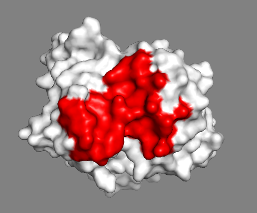
Identifying the paratope of the antibody
Nowadays several computational tools can identify the paratope (the residues of the hypervariable loops involved in binding) from the provided antibody sequence. In this tutorial, we are providing you with the corresponding list of residue obtained using ProABC-2. ProABC-2 uses a convolutional neural network to identify not only residues which are located in the paratope region but also the nature of interactions they are most likely involved in (hydrophobic or hydrophilic). The work is described in Ambrosetti, et al Bioinformatics, 2020.
The corresponding paratope residues (those with either an overall probability >= 0.4 or a probability for hydrophobic or hydrophilic > 0.3) are:
31,32,33,34,35,52,54,55,56,100,101,102,103,104,105,106,151,152,169,170,173,211,212,213,214,216
The numbering corresponds to the numbering of the 4G6K_clean.pdb PDB file.
Let us visualize those onto the 3D structure.
For this start PyMOL and load 4G6K_clean.pdb
File menu -> Open -> select 4G6K_clean.pdb
Alternatively, if PyMOL is accessible from the command line, simply type:
We will now highlight the predicted paratope residues in red. In PyMOL type the following commands:
Let us now switch to a surface representation to inspect the predicted binding site.
Inspect the surface.
Do the identified paratope residues form a well-defined patch on the surface?
See surface view of the paratope expand_more
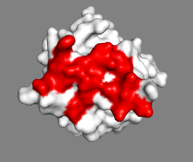
Identifying the epitope of the antigen
The article describing the crystal structure of the antibody-antigen complex we are modeling also reports experimental NMR chemical shift titration experiments to map the binding site of the antibody (gevokizumab) on Interleukin-1β. The residues affected by binding are listed in Table 5 of Blech et al. JMB 2013:
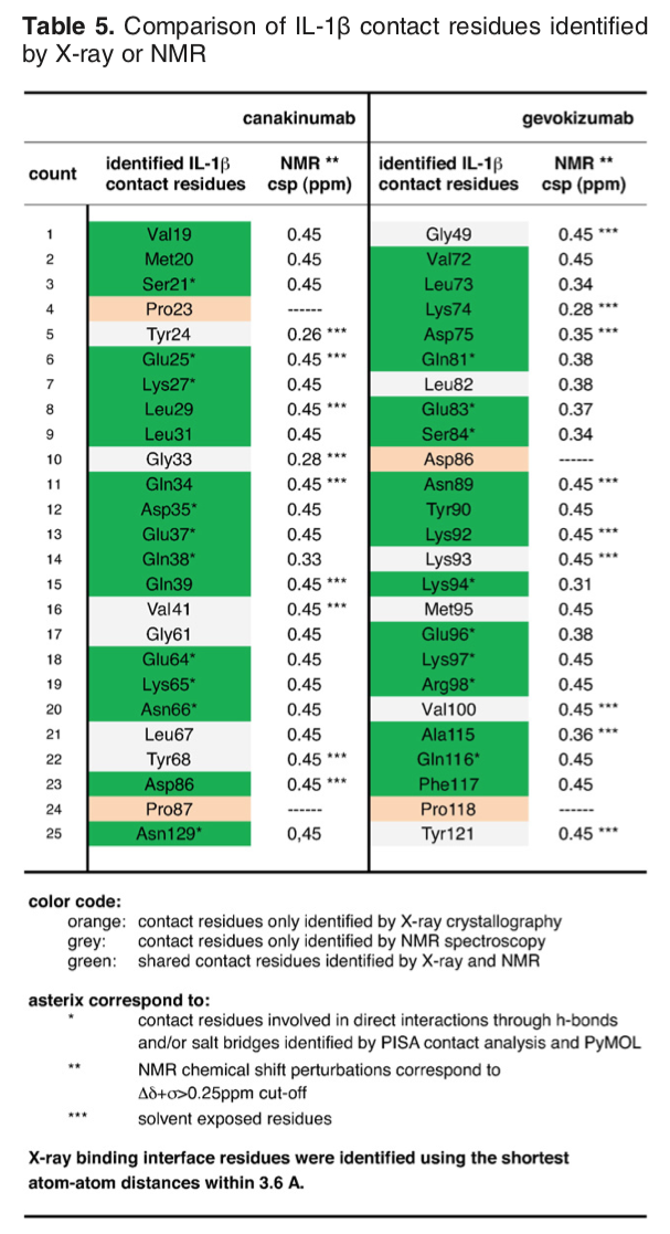
The list of binding site (epitope) residues identified by NMR is:
72,73,74,75,81,83,84,89,90,92,94,96,97,98,115,116,117
We will now visualize the epitope on Interleukin-1β. To do this, start PyMOL and open the provided PDB file of the antigen from the PyMOL File menu.
File menu -> Open -> select 4I1B_clean.pdb
Inspect the surface.
Do the identified residues form a well-defined patch on the surface?
The answer to that question should be yes, but we can see some residues not colored that might also be involved in the binding - there are some white spots around/in the red surface.
See surface view of the epitope identified by NMR expand_more
In HADDOCK, we are dealing with potentially incomplete binding sites by defining surface neighbors as passive residues.
These passive residues are added in the definition of the interface but do not incur any energetic penalty if they are not part of the binding site in the final models.
In contrast, residues defined as active (typically the identified or predicted binding site residues) will incur an energetic penalty.
When using the HADDOCK2.x webserver, passive residues will be automatically defined.
Here, since we are using a local version, we need to define those manually.
This can easily be done using a haddock3 command line tool in the following way:
The command prints a list of solvent accessible passive residues, which you should save to a file for further use.
We can visualize the epitope and its surface neighbors using PyMOL:
File menu -> Open -> select 4I1B_clean.pdb
See the epitope and passive residues expand_more
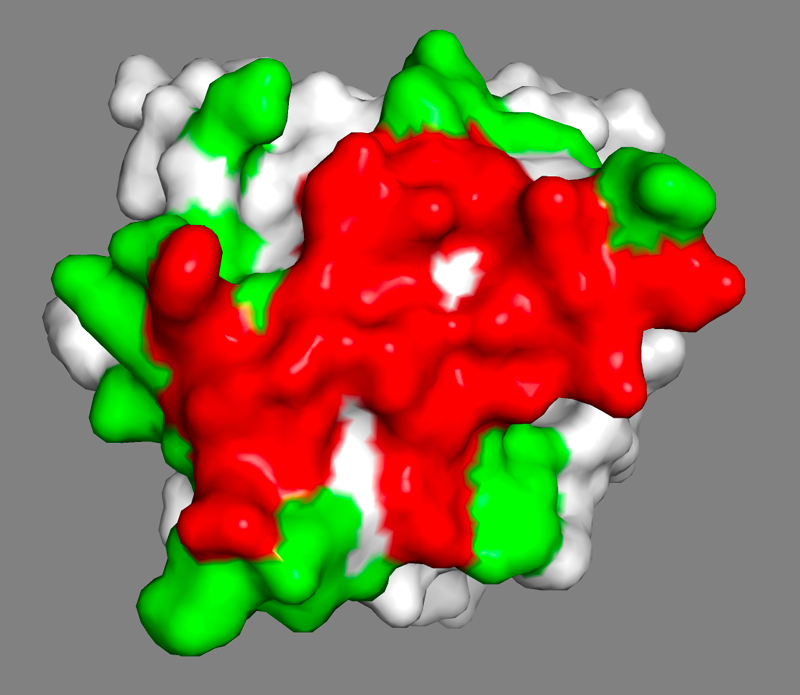
The NMR-identified residues and their surface neighbors generated with the above command can be used to define ambiguous interactions restraints, either using the NMR identified residues as active in HADDOCK, or combining those with the surface neighbors.
The difference between active and passive residues in HADDOCK is as follows:
Active residues: These residues are “forced” to be at the interface. If they are not part of the interface in the final models, an energetic penalty will be applied. The interface in this context is defined by the union of active and passive residues on the partner molecules.
Passive residues: These residues are expected to be at the interface. However, if they are not, no energetic penalty is applied.
In general, it is better to be too generous rather than too strict in the definition of passive residues.
An important aspect is to filter both the active (the residues identified from your mapping experiment) and passive residues by their solvent accessibility.
This is done automatically when using the haddock3-restraints passive_from_active command: residues with less that 15% relative solvent accessibility (same cutoff as the default in the HADDOCK server) are discared.
This is, however, not a hard limit, and you might consider including even more buried residues if some important chemical group seems solvent accessible from a visual inspection.
Defining ambiguous restraints
Once you have identified your active and passive residues for both molecules, you can proceed with the generation of the ambiguous interaction restraints (AIR) file for HADDOCK.
For this you can either make use of our online Generate Restraints haddock-restraints web service, entering the list of active and passive residues for each molecule,
the chainIDs of each molecule and saving the resulting restraint list to a text file, or use another haddock3-restraints sub-command.
To use our haddock3-restraints active_passive_to_ambig script, you need to
create for each molecule a file containing two lines:
- The first line corresponds to the list of active residues (numbers separated by spaces)
- The second line corresponds to the list of passive residues (numbers separated by spaces).
Important: The file must consist of two lines, but a line can be empty (e.g., if you do not want to define active residues for one molecule). However, there must be at least one set of active residue defined for one of the molecules.
- For the antibody we will use the predicted paratope as active and no passive residues defined.
The corresponding file can be found in the
restraintsdirectory asantibody-paratope.act-pass:
1 32 33 34 35 52 54 55 56 100 101 102 103 104 105 106 151 152 169 170 173 211 212 213 214 216
- For the antigen we will use the NMR-identified epitope as active and the surface neighbors as passive.
The corresponding file can be found in the
restraintsdirectory asantigen-NMR-epitope.act-pass:
72 73 74 75 81 83 84 89 90 92 94 96 97 98 115 116 117
3 24 46 47 48 50 66 76 77 79 80 82 86 87 88 91 93 95 118 119 120
Using those two files, we can generate the CNS-formatted Ambiguous Interaction Restraints (AIRs) file with the following command:
This generates a file called ambig-paratope-NMR-epitope.tbl that contains the AIRs.
Inspect the generated file and note how the ambiguous distances are defined.
View an extract of the AIR file expand_more
assign (resi 31 and segid A)
(
       (resi 72 and segid B)
        or
       (resi 73 and segid B)
        or
       (resi 74 and segid B)
        or
       (resi 75 and segid B)
        or
       (resi 81 and segid B)
        or
       (resi 83 and segid B)
        or
       (resi 84 and segid B)
        or
       (resi 89 and segid B)
        or
       (resi 90 and segid B)
        or
       (resi 92 and segid B)
        or
       (resi 94 and segid B)
        or
       (resi 96 and segid B)
        or
       (resi 97 and segid B)
        or
       (resi 98 and segid B)
        or
       (resi 115 and segid B)
        or
       (resi 116 and segid B)
        or
       (resi 117 and segid B)
        or
       (resi 3 and segid B)
        or
       (resi 24 and segid B)
        or
       (resi 46 and segid B)
        or
       (resi 47 and segid B)
        or
       (resi 48 and segid B)
        or
       (resi 50 and segid B)
        or
       (resi 66 and segid B)
        or
       (resi 76 and segid B)
        or
       (resi 77 and segid B)
        or
       (resi 79 and segid B)
        or
       (resi 80 and segid B)
        or
       (resi 82 and segid B)
        or
       (resi 86 and segid B)
        or
       (resi 87 and segid B)
        or
       (resi 88 and segid B)
        or
       (resi 91 and segid B)
        or
       (resi 93 and segid B)
        or
       (resi 95 and segid B)
        or
       (resi 118 and segid B)
        or
       (resi 119 and segid B)
        or
       (resi 120 and segid B)
) 2.0 2.0 0.0
...
See answer expand_more
The default distance range for those is between 0 and 2Å, which might seem short but makes senses because of the 1/r^6 summation in the AIR energy function that makes the effective distance to be significantly shorter than the shortest distance entering the sum.The effective distance is calculated as the SUM over all pairwise atom-atom distance combinations between an active residue and all the active+passive on the other molecule: SUM[1/r^6]^(-1/6).
Restraints validation
If you modify manually this generated restraint files or create your own, it is possible to quickly check if the format is valid using the following haddock3-restraints sub-command:
haddock3-restraints validate_tbl ambig-paratope-NMR-epitope.tbl --silent
No output means that your TBL file is valid.
Note that this only validates the syntax of the restraint file, but does not check if the selections defined in the restraints are actually existing in your input PDB files.
Additional restraints for multi-chain proteins
As an antibody consists of two separate chains, it is important to define a few distance restraints
to keep them together during the high temperature flexible refinement stage of HADDOCK otherwise they might slightly drift appart.
This can easily be done using the haddock3-restraints restrain_bodies sub-command.
haddock3-restraints restrain_bodies 4G6K_clean.pdb > antibody-unambig.tbl
The result file contains two CA-CA distance restraints with the exact distance measured between two randomly picked CA atoms pairs:
  assign (segid A and resi 110 and name CA) (segid A and resi 132 and name CA) 26.326 0.0 0.0
  assign (segid A and resi 97 and name CA) (segid A and resi 204 and name CA) 19.352 0.0 0.0
This file is also provided in the restraints directory.
Setting up and running the docking with HADDOCK3
Now that we have all required files at hand (PDB and restraints files), it is time to setup our docking protocol. In this tutorial, considering we have rather good information about the paratope and epitope, we will execute a fast HADDOCK3 docking workflow, reducing the non-negligible computational cost of HADDOCK by decreasing the sampling, without impacting too much the accuracy of the resulting models.
HADDOCK3 workflow definition
The first step is to create a HADDOCK3 configuration file that will define the docking workflow. We will follow a classic HADDOCK workflow consisting of rigid body docking, semi-flexible refinement and final energy minimisation followed by clustering.
We will also integrate two analysis modules in our workflow:
caprievalwill be used at various stages to compare models to either the best scoring model (if no reference is given) or a reference structure, which in our case we have at hand (pdbs/4G6M_matched.pdb). This will directly allow us to assess the performance of the protocol. In the absence of a reference,caprievalis still usefull to assess the convergence of a run and analyse the results.contactmapadded as last module will generate contact matrices of both intra- and intermolecular contacts and a chordchart of intermolecular contacts for each cluster.
Our workflow consists of the following modules:
topoaa: Generates the topologies for the CNS engine and builds missing atomsrigidbody: Performs rigid body energy minimisation (it0in haddock2.x)caprieval: Calculates CAPRI metrics (i-RMSD, l-RMSD, Fnat, DockQ) with respect to the top scoring model or reference structure if providedseletop: Selects the top X models from the previous moduleflexref: Preforms semi-flexible refinement of the interface (it1in haddock2.4)caprievalemref: Final refinement by energy minimisation (itwEM only in haddock2.4)caprievalclustfcc: Clustering of models based on the fraction of common contacts (FCC)seletopclusts: Selects the top models of all clusterscaprievalcontactmap: Contacts matrix and a chordchart of intermolecular contacts
The corresponding toml configuration file (provided in workflows/docking-antibody-antigen.cfg) looks like:
# ====================================================================
# Antibody-antigen docking example with restraints from the antibody
# paratope to the NMR-identified epitope on the antigen
# ====================================================================

# Directory in which the scoring will be done
run_dir = "run1"

# Compute mode
mode = "local"
ncores = 50

# Self contained rundir (to avoid problems with long filename paths)
self_contained = true

# Post-processing to generate statistics and plots
postprocess = true
clean = true

molecules =  [
    "pdbs/4G6K_clean.pdb",
    "pdbs/4I1B_clean.pdb"
    ]

# ====================================================================
# Parameters for each stage are defined below, prefer full paths
# ====================================================================
[topoaa]

[rigidbody]
# CDR to NMR epitope ambig restraints
ambig_fname = "restraints/ambig-paratope-NMR-epitope.tbl"
# Restraints to keep the antibody chains together
unambig_fname = "restraints/antibody-unambig.tbl"
# Reduced sampling (100 instead of the default of 1000)
sampling = 100

[caprieval]
reference_fname = "pdbs/4G6M_matched.pdb"

[seletop]
# Selection of the top 50 best scoring complexes (instead of the default of 200)
select = 50

[flexref]
tolerance = 5
# CDR to NMR epitope ambig restraints
ambig_fname = "restraints/ambig-paratope-NMR-epitope.tbl"
# Restraints to keep the antibody chains together
unambig_fname = "restraints/antibody-unambig.tbl"

[caprieval]
reference_fname = "pdbs/4G6M_matched.pdb"

[emref]
tolerance = 5
# CDR to NMR epitope ambig restraints
ambig_fname = "restraints/ambig-paratope-NMR-epitope.tbl"
# Restraints to keep the antibody chains together
unambig_fname = "restraints/antibody-unambig.tbl"

[caprieval]
reference_fname = "pdbs/4G6M_matched.pdb"

[clustfcc]
plot_matrix = true

[seletopclusts]
# Selection of the top 4 best scoring complexes from each cluster
top_models = 4

[caprieval]
reference_fname = "pdbs/4G6M_matched.pdb"

[contactmap]

# ====================================================================
In this case, since we have information for both interfaces we use a low-sampling configuration file, which takes only a small amount of computational resources to run.
The initial sampling parameter at the rigid-body energy minimization (rigidbody) module is set to 100 models, of which only best the 40 are passed to the flexible refinement (flexref) module with the seletop module.
The subsequence flexible refinement (flexref module) and energy minimisation (emref) modules will use all models passed by the seletop module.
FCC clustering (clustfcc) is then applied to group together models sharing a consistent fraction of the interface contacts.
The top 4 models of each cluster are saved to disk (seletopclusts).
Multiple caprieval modules are executed at different stages of the workflow to check how the quality (and rankings) of the models change throughout the protocol.
In this case we are providing the known crystal structure of the complex as reference.
Note: For making best use of the available CPU resources it is recommended to adapt the sampling parameter to be a multiple of the number of available cores when running in local mode. For this reason, for the ASM HPC/AI school the sampling is set to be a multiple of 48.
Note: In case no reference is available (the usual scenario), the best ranked model is used as reference for each stage.
Including caprieval at the various stages even when no reference is provided is useful to get the rankings and scores and visualise the results (see Analysis section below).
Note: The default sampling would be 1000 models for rigidbody of which 200 are passed to the flexible refinement in seletop.
As an indication of the computational requirements, the default sampling worflow for this tutorial completes in about 37min using 12 cores on a MaxOSX M2 processor.
In comparison, the reduced sampling run (100/40) takes about 7-8min.
Note: To get a list of all possible parameters that can be defined in a specific module (and their default values) you can use the following command:
Add the -d option to get a more detailed description of parameters and use the -h option to see a list of arguments and options.
Alternatively, you can consult the developer’s guide, where each parameter of each module is listed along with their default values, short and long descriptions, etc. Navigate to the Modules and select a module which parameters you want to display.
Note that, in contrast to HADDOCK2.X, we have much more flexibility in defining our workflow. As an example, we could use this flexibility by introducing a clustering step after the initial rigid-body docking stage, selecting a given number of models per cluster and refining all of those. For an example of this strategy see the 4 section about ensemble docking.
Running HADDOCK3
In in the first section of the workflow above we have a parameter mode defining the execution mode. HADDOCK3 currently supports three difference execution modes:
- local : In this mode, HADDOCK3 will run on the current system, using the defined number of cores (
ncores) in the config file to a maximum of the total number of available cores on the system. - batch: In this mode, HADDOCK3 will typically be started on your local server (e.g. the login node) and will dispatch jobs to the batch system of your cluster (slurm and torque are currently supported).
- mpi: HADDOCK3 also supports a pseudo parallel MPI implementation, which allows to harvest the power of multiple nodes to distribute the computations (functional but still very experimental at this stage).
Execution of HADDOCK3 on the computers of the BioExcel 2026 summerschool
To execute the HADDOCK3 workflow on the computational resources provided for this workshop, we will simply run in local mode, calling haddock3 with as argument the workflow you want to execute.
haddock3 <my-workflow-configuration-file>Alternatively redirect the output to a log file and send haddock3 to the background.
As an indication, running locally on an Apple M2 laptop using 10 cores, this workflow completed in 7 minutes. On the laptops used for the BioExcel summerschool, the execution time should be about 9 minutes.
Execution of HADDOCK3 on DISCOVERER (BioExcel Sofia May 2025 workshop)
View execution instructions for running HADDOCK3 on DISCOVERER expand_more
To execute the HADDOCK3 workflow on the computational resources provided for this workshop, you should create an execution script contain specific requirements for the queueing system and the HADDOCK3 configuration and execution. An example slurm script is provided with the data you unzipped:run-haddock3-discoverer.sh#!/bin/bash
#SBATCH --nodes=1
#SBATCH --account=school-01
#SBATCH --qos=school-01
#SBATCH --job-name "haddock3"
#SBATCH --tasks-per-node=50
#SBATCH --mem-per-cpu 1500
#SBATCH --time 04:00:00
module load python/3/3.12
module load haddock3/2025.5.0
haddock3 workflows/docking-antibody-antigen.cfgExecution of HADDOCK3 on the TRUBA resources (EuroCC Istanbul April 2024 workshop)
View execution instructions for running HADDOCK3 the TRUBA resources expand_more
To execute the HADDOCK3 workflow on the computational resources provided for this workshop, you should create an execution script contain specific requirements for the queueing system and the HADDOCK3 configuration and execution. Two scripts are provided with the data you unzipped, one for execution on the hamsri cluster and one for the barbun cluster:run-haddock3-barbun.sh
run-haddock3-hamsri.sh#!/bin/bash
#SBATCH --nodes=1
#SBATCH --tasks-per-node=54
#SBATCH -C weka
#SBATCH -p hamsi
#SBATCH --time 00:30:00
source ~egitim/HADDOCK/haddock3/.venv/bin/activate
haddock3 workflows/docking-antibody-antigen.cfgsbatch run-haddock3-hamsri.shExecution of HADDOCK3 on Fugaku (ASM 2026 HPC/AI school, Kobe Japan)
View execution instructions for running HADDOCK3 on Fugaku expand_more
To execute the workflow on Fugaku, you can either start an interactive session or create a job file that will execute HADDOCK3 on a node, with HADDOCK3 running in local mode (the setup in the above configuration file with mode="local") and harvesting all core of that node (ncores=48).Interactive session on a node:
pjsub -x PJM_LLIO_GFSCACHE=/vol0003:/vol0004 -g "hp250477" --interact -L "node=1" - -L "rscgrp=int" -L "elapse=2:00:00" --sparam "wait-time=600"source /vol0300/data/hp250477/Materials/Life_Science/20250202_Bonvin/haddock3/.venv/bin/activate<br>haddock3 ./workflows/docking-antibody-antigen.cfgFor this execution mode you should create an execution script contain specific requirements for the queueing system and the HADDOCK3 configuration and execution. Here is an example of such an execution script (also provided in the HADDOCK3-antibody-antigen directory as run-haddock3-fugaku.sh):
#!/bin/sh -x
#PJM -L  "node=1"                           # Assign node 1 node
#PJM -L  "rscgrp=small"                     # Specify resource group
#PJM -L  "elapse=02:00:00"                  # Elapsed time limit 1 hour
#PJM -g hp250477                            # group name
#PJM -x PJM_LLIO_GFSCACHE=/vol0003:/vol0004 # volume names that job uses
#PJM -s                                     # Statistical information output

source /vol0300/data/hp250477/Materials/Life_Science/20260202-HADDOCK/haddock3/.venv/bin/activate
haddock3 ./workflows/docking-antibody-antigen.cfgpjsub run-haddock3-fugaku.shAnd you can check the status in the queue using pjstat. This run should take about 25 minutes to complete on a single node using 48 arm cores.
Execution of HADDOCK3 on ADD Ljubljana (BioExcel Adriatic edition 2026, Ljubljana, Slovenia)
View execution instructions for running HADDOCK3 on the ADD cluster expand_more
To execute the workflow, you can either start an interactive session or create a job file that will execute HADDOCK3 on a node, with HADDOCK3 running in local mode (the setup in the above configuration file with mode="local") and harvesting all core of that node (ncores=16).Start an interactive session on a node:
salloc --job-name=interactive_haddock3 --partition=amd --nodes=1 --cpus-per-task=16 --time-min=120source /home/vreys/haddock3/.haddock3-env/bin/activate<br>haddock3 ./workflows/docking-antibody-antigen.cfgFor this execution mode you should create an execution script contain specific requirements for the queueing system and the HADDOCK3 configuration and execution. Here is an example of such an execution script (that can be saved under the name run-haddock3-slurm.sh):
#!/bin/bash
#SBATCH --partition=amd
#SBATCH --job-name=haddock3_run
#SBATCH --nodes=1
#SBATCH --cpus-per-task=16
#SBATCH --time-min=120
#SBATCH --output="haddock3_run_log.txt"

# Source the environement
source /home/vreys/haddock3/.haddock3-env/bin/activate

# Go to the appropriate directory
cd ~/HADDOCK3-antibody-antigen

# Launch haddock3
haddock3 workflows/docking-antibody-antigen.cfgsbatch run-haddock3-slurm.shAnd you can check the status in the queue using squeue -u Username. Also, you can follow the state of your run by looking a the content of either the log file or the slurm output using:
tail -f haddock3_run_log.txtLearn more about the various execution modes of haddock3
Local execution expand_more
In this mode HADDOCK3 will run on the current system, using the defined number of cores (ncores) in the config file to a maximum of the total number of available cores on the system minus one. An example of the relevant parameters to be defined in the first section of the config file is:# compute mode
mode = "local"
# 1 nodes x 50 ncores
ncores = 50haddock3 <my-workflow-configuration-file>haddock3 <my-workflow-configuration-file> > haddock3.log &Exection in batch mode using slurm expand_more
Here is an example script for submitting via the slurm batch system:#!/bin/bash
#SBATCH --nodes=1
#SBATCH --tasks-per-node=50
#SBATCH -J haddock3
#SBATCH --partition=medium
# activate the haddock3 conda environment
source $HOME/miniconda3/etc/profile.d/conda.sh
conda activate haddock3
# go to the run directory
cd $HOME/HADDOCK3-antibody-antigen
# execute
haddock3 <my-workflow-configuration-file>In this mode HADDOCK3 will typically be started on your local server (e.g. the login node) and will dispatch jobs to the batch system of your cluster. Two batch systems are currently supported: slurm and torque (defined by the batch_type parameter). In the configuration file you will have to define the queue name and the maximum number of concurrent jobs sent to the queue (queue_limit). Since HADDOCK3 single model calculations are quite fast, it is recommended to calculate multiple models within one job submitted to the batch system. he number of model per job is defined by the concat parameter in the configuration file. You want to avoid sending thousands of very short jobs to the batch system if you want to remain friend with your system administrators... An example of the relevant parameters to be defined in the first section of the config file is:
  # compute mode
  mode = "batch"
  # batch system
  batch_type = "slurm"
  # queue name
  queue = "short"
  # number of concurrent jobs to submit to the batch system
  queue_limit = 100
  # number of models to produce per submitted job
  concat = 10
Exection in MPI mode expand_more
HADDOCK3 supports a parallel pseudo-MPI implementation. For this to work, the mpi4py library must have been installed at installation time. Refer to the (MPI-related instructions). The execution mode should be set to `mpi` and the total number of cores should match the requested resources when submitting to the batch system. An example of the relevant parameters to be defined in the first section of the config file is:# compute mode
mode = "mpi"
# 5 nodes x 50 tasks = ncores = 250
ncores = 250 #!/bin/bash
#SBATCH --nodes=5
#SBATCH --tasks-per-node=50
#SBATCH -J haddock3mpi
# Make sure haddock3 is activated
source $HOME/miniconda3/etc/profile.d/conda.sh
conda activate haddock3
# go to the run directory
# edit if needed to specify the correct location
cd $HOME/HADDOCK3-antibody-antigen
# execute
haddock3 \<my-workflow-configuration-file\>
Analysis of docking results
In case something went wrong with the docking (or simply if you do not want to wait for the results) you can find the following precalculated runs in the runs directory:
run1: docking run created using the unbound antibody.run-energetics-alascan: Alanine scanning of the interface (see Bonus 1)run1-af2: docking run created using the Alphafold-multimer antibody (see Bonus 3).run1-abb: docking run created using the Immunebuilder antibody (see Bonus 3).run1-ens: docking run created using an ensemble of antibody models (see Bonus 4).run-scoring: scoring run created using various models obtained at the previous stages (see Bonus 6).
Once your run has completed - inspect the content of the resulting directory. You will find the various steps (modules) of the defined workflow numbered sequentially starting at 0, e.g.:
> ls run1/
     00_topoaa/
     01_rigidbody/
     02_caprieval/
     03_seletop/
     04_flexref/
     05_caprieval/
     06_emref/
     07_caprieval/
     08_clustfcc/
     09_seletopclusts/
     10_caprieval/
     11_contactmap/
     analysis/
     data/
     log
     toppar/
     traceback/
In addition, there is a log file (text file) and four additional directories:
- the
analysisdirectory contains various plots to visualize the results for each caprieval step and a general report (report.html) that provides all statistics with various plots. You can open this file in your preferred web browser - the
datadirectory contains the input data (PDB and restraint files) for the various modules, as well as an input workflow (inconfigurationsdirectory) - the
toppardirectory contains the force field topology and parameter files (only present when running in self-contained mode) - the
tracebackdirectory containstraceback.tsv, which links all models to see which model originates from which throughout all steps of the workflow.
You can find information about the duration of the run at the bottom of the log file.
Each sampling/refinement/selection module will contain PDB files.
For example, the 09_seletopclusts directory contains the selected models from each cluster. The clusters in that directory are numbered based
on their rank, i.e. cluster_1 refers to the top-ranked cluster. Information about the origin of these files can be found in that directory in the seletopclusts.txt file.
The simplest way to extract ranking information and the corresponding HADDOCK scores is to look at the XX_caprieval directories (which is why it is a good idea to have it as the final module, and possibly as intermediate steps). This directory will always contain a capri_ss.tsv single model statistics file, which contains the model names, rankings and statistics (score, iRMSD, Fnat, lRMSD, ilRMSD and dockq score). E.g. for 10_caprieval:
model   md5     caprieval_rank  score   irmsd   fnat    lrmsd   ilrmsd  dockq   rmsd    cluster_id      cluster_ranking model-cluster_ranking   air       angles  bonds   bsa     cdih    coup    dani    desolv  dihe    elec    improper        rdcs    rg      sym     total   vdw     vean    xpcs
../09_seletopclusts/cluster_1_model_1.pdb       -       1       -141.456        1.287   0.759   3.004   2.442   0.741   1.294   1       1       1         81.228  283.732 53.892  1861.960        0.000   0.000   0.000   6.600   2046.800        -534.635        78.164  0.000   0.000   0.000   -502.659  -49.252 0.000   0.000
../09_seletopclusts/cluster_1_model_2.pdb       -       2       -139.593        0.805   0.931   1.390   1.069   0.894   0.880   1       1       2         145.313 285.685 54.305  1882.540        0.000   0.000   0.000   0.298   2044.710        -536.474        74.008  0.000   0.000   0.000   -438.288  -47.127 0.000   0.000
../09_seletopclusts/cluster_1_model_3.pdb       -       3       -133.609        0.871   0.897   1.777   1.540   0.868   0.858   1       1       3         99.629  271.913 53.934  1879.650        0.000   0.000   0.000   3.322   2033.770        -504.554        74.324  0.000   0.000   0.000   -450.908  -45.983 0.000   0.000
../09_seletopclusts/cluster_1_model_4.pdb       -       4       -129.384        1.026   0.828   2.049   1.909   0.818   0.984   1       1       4         134.222 279.400 52.383  1963.630        0.000   0.000   0.000   6.498   2042.270        -528.330        74.056  0.000   0.000   0.000   -437.746  -43.638 0.000   0.000
../09_seletopclusts/cluster_2_model_1.pdb       -       5       -125.011        4.957   0.138   11.775  10.850  0.188   4.257   2       2       1         102.261 298.251 53.578  1611.600        0.000   0.000   0.000   2.229   2039.950        -309.326        77.663  0.000   0.000   0.000   -282.666  -75.601 0.000   0.000
...
If clustering was performed prior to calling the caprieval module, the capri_ss.tsv file will also contain information about to which cluster the model belongs to and its ranking within the cluster.
The relevant statistics are:
- score: the HADDOCK score (arbitrary units)
- irmsd: the interface RMSD, calculated over the interfaces the molecules
- fnat: the fraction of native contacts
- lrmsd: the ligand RMSD, calculated on the ligand after fitting on the receptor (1st component)
- ilrmsd: the interface-ligand RMSD, calculated over the interface of the ligand after fitting on the interface of the receptor (more relevant for small ligands for example)
- dockq: the DockQ score, which is a combination of irmsd, lrmsd and fnat and provides a continuous scale between 1 (exactly equal to reference) and 0
Various other terms are also reported including:
- bsa: the buried surface area (in squared angstroms)
- elec: the intermolecular electrostatic energy
- vdw: the intermolecular van der Waals energy
- desolv: the desolvation energy
The iRMSD, lRMSD and Fnat metrics are the ones used in the blind protein-protein prediction experiment CAPRI (Critical PRediction of Interactions).
In CAPRI the quality of a model is defined as (for protein-protein complexes):
- acceptable model: i-RMSD < 4Å or l-RMSD < 10Å and Fnat > 0.1 (0.23 < DOCKQ < 0.49)
- medium quality model: i-RMSD < 2Å or l-RMSD < 5Å and Fnat > 0.3 (0.49 < DOCKQ < 0.8)
- high quality model: i-RMSD < 1Å or l-RMSD < 1Å and Fnat > 0.5 (DOCKQ > 0.8)
In case where the caprieval module is called after a clustering step, an additional capri_clt.tsv file will be present in the directory.
This file contains the cluster ranking and score statistics, averaged over the minimum number of models defined for clustering
(4 by default), with their corresponding standard deviations. E.g.:
cluster_rank    cluster_id  n   under_eval  score   score_std  irmsd   irmsd_std   fnat   fnat_std   lrmsd   lrmsd_std  dockq   dockq_std  ilrmsd  ilrmsd_std  rmsd    rmsd_std    air air_std bsa bsa_std desolv  desolv_std  elec    elec_std    total   total_std   vdw vdw_std caprieval_rank
1       1       4       -       -136.011         4.800    0.997   0.185   0.853   0.066    2.055  0.596   0.830   0.058    1.740  0.503    1.004   0.174   115.098 25.812  1896.945        39.298  4.179   2.600   -525.998        12.744  -457.400        26.656  -46.500 2.026   1
2       2       4       -       -104.584        12.107    4.982   0.020   0.138   0.012   11.875  0.400   0.187   0.008   10.761  0.133    4.421   0.100   157.628 41.066  1615.062        33.866  5.497   2.482   -287.197        33.869  -197.974        61.736  -68.405 7.598   2
3       3       4       -        -90.483         4.847   10.254   0.504   0.078   0.015   19.491  0.651   0.086   0.009   18.142  0.520   10.577   0.572   162.792 39.855  1530.568        47.235  4.521   1.864   -361.098        46.709  -237.370        45.213  -39.064 8.018   3
In this file you find the cluster rank (which corresponds to the naming of the clusters in the previous seletop directory), the cluster ID (which is related to the size of the cluster, 1 being always the largest cluster), the number of models (n) in the cluster and the corresponding statistics (averages + standard deviations). The corresponding cluster PDB files will be found in the preceeding 09_seletopclusts directory.
While these simple text files can be easily checked from the command line already, they might be cumbersome to read.
For that reason, we have developed a post-processing analysis that automatically generates html reports for all caprieval steps in the workflow.
These are located in the respective analysis/XX_caprieval directories and can be viewed using your favorite web browser.
Cluster statistics
Let us now analyse the docking results. Use for that either your own run or a pre-calculated run provided in the runs directory.
Go into the analysis/10_caprieval_analysis directory of the respective run directory (if needed copy the run or that directory to your local computer) and open in a web browser the report.html file. Be patient as this page contains interactive plots that may take some time to generate.
On the top of the page, you will see a table that summarises the cluster statistics (taken from the capri_clt.tsv file).
The columns (corresponding to the various clusters) are sorted by default on the cluster rank, which is based on the HADDOCK score (found on the 4th row of the table).
As this is an interactive table, you can sort it as you wish by using the arrows present in the first column.
Simply click on the arrows of the term you want to use to sort the table (and you can sort it in ascending or descending order).
A snapshot of this table is shown below:
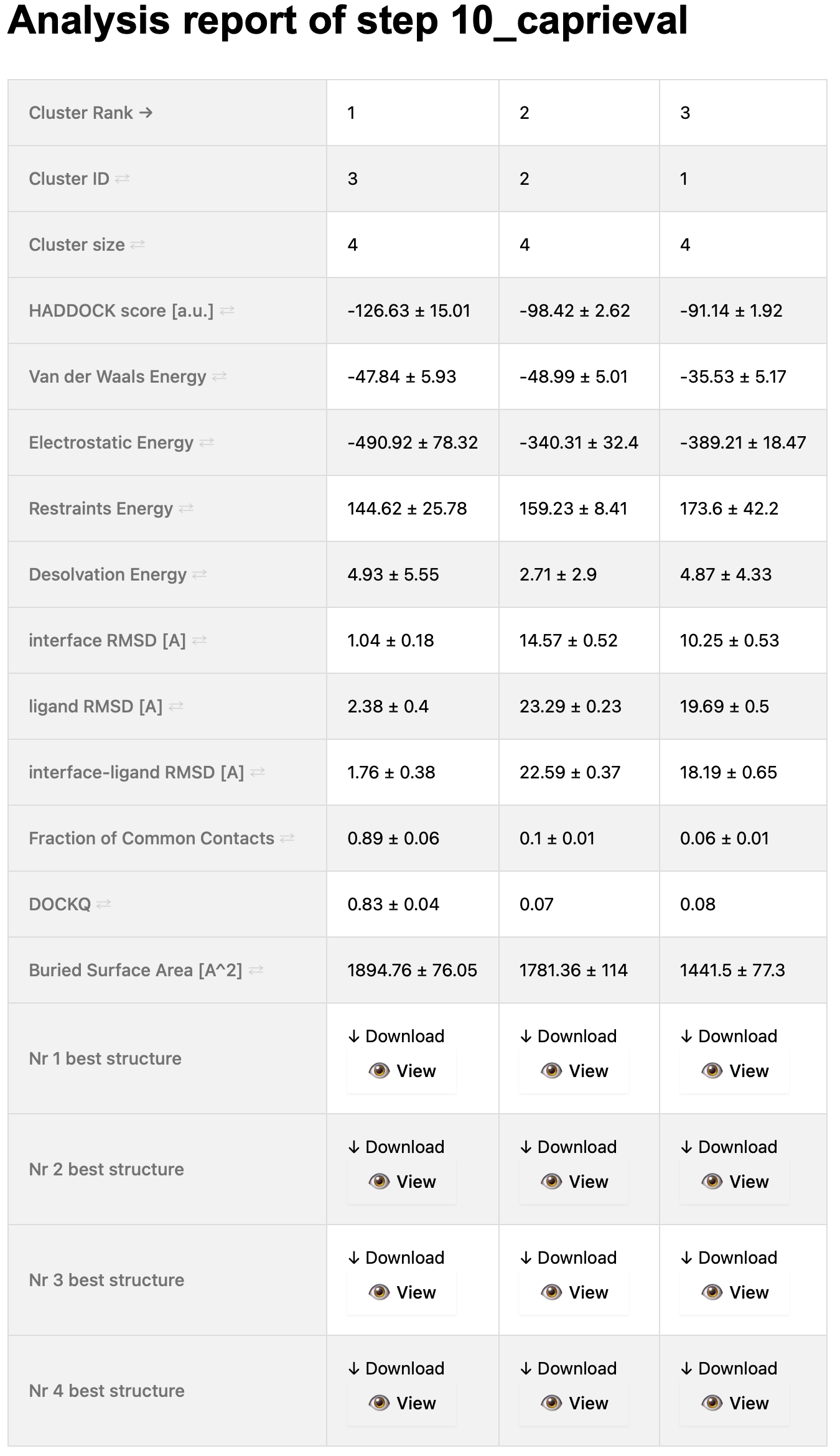
You can also view this report online here
Note that in case the PDB files are still compressed (gzipped) the download links will not work. Also online visualisation is not enabled. To overcome this disk space storge solution, consider adding the global parameter clean = true at the begining of your configuration file.
Inspect the final cluster statistics
How many clusters have been generated?
Since for this tutorial we have at hand the crystal structure of the complex, we provided it as reference to the caprieval modules.
This means that the iRMSD, lRMSD, Fnat and DockQ statistics report on the quality of the docked model compared to the reference crystal structure.
How many clusters of acceptable or better quality have been generate according to CAPRI criteria?
What is the rank of the best cluster generated?
What is the rank of the first acceptable of better cluster generated?
Visualizing the scores and their components
Next to the cluster statistic table shown above, the report.html file also contains a variety of plots displaying the HADDOCK score
and its components against various CAPRI metrics (i-RMSD, l-RMSD, Fnat, Dock-Q) with a color-coded representation of the clusters.
These are interactive plots. A menu on the top right of the first row (you might have to scroll to the rigth to see it)
allows you to zoom in and out in the plots and turn on and off clusters.
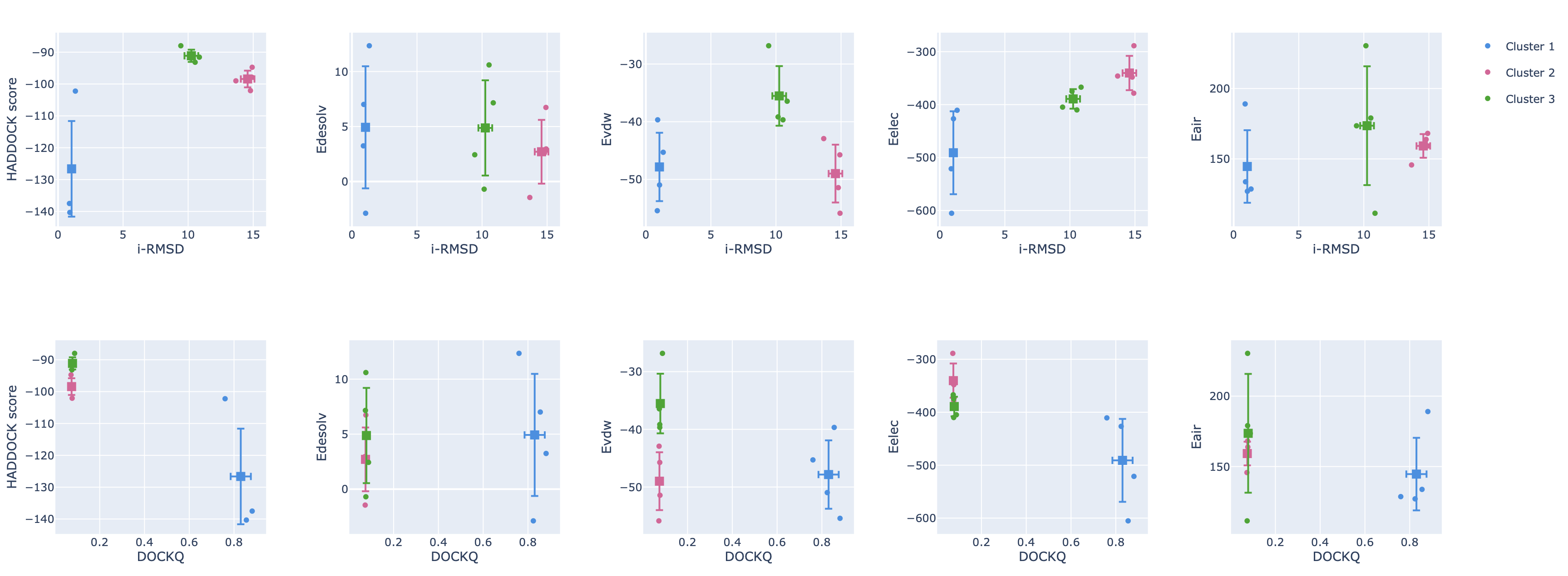
As a reminder, you can also view this report online here
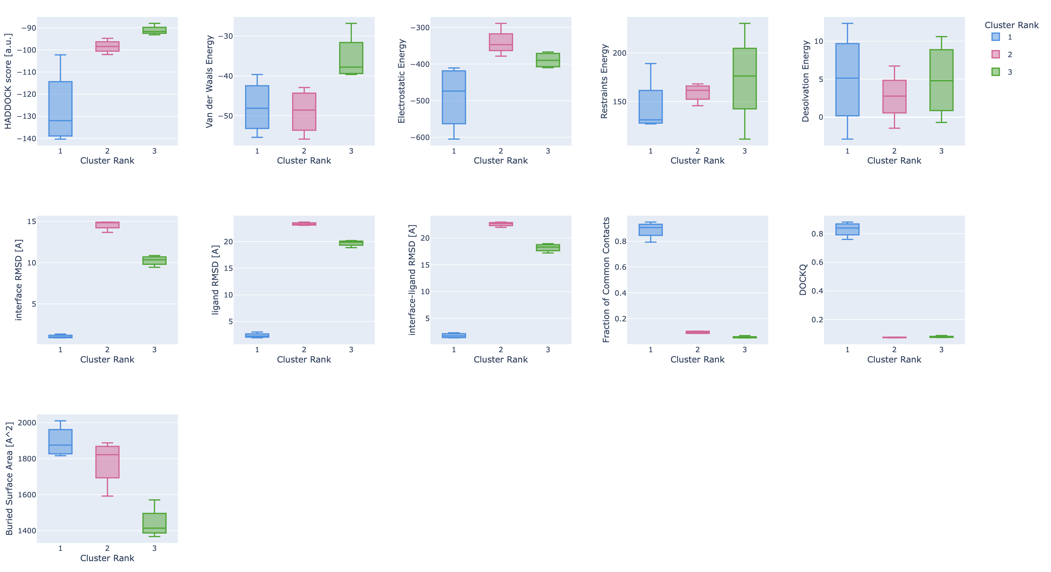
Finally, the report also shows plots of the cluster statistics (distributions of values per cluster ordered according to their HADDOCK rank):
Some single structure analysis
Going back to command line analysis, we are providing in the scripts directory a simple script that extracts some model statistics for acceptable or better models from the caprieval steps.
To use it, simply call the script with as argument the run directory you want to analyze, e.g.:
./scripts/extract-capri-stats.sh ./runs/run1
View the output of the script expand_more
==============================================
== run1/02_caprieval/capri_ss.tsv
==============================================
Total number of acceptable or better models:  18  out of  100
Total number of medium or better models:      12  out of  100
Total number of high quality models:          2  out of  100

First acceptable model - rank:  2  i-RMSD:  1.221  Fnat:  0.776  DockQ:  0.766
First medium model     - rank:  2  i-RMSD:  1.221  Fnat:  0.776  DockQ:  0.766
Best model             - rank:  19  i-RMSD:  0.966  Fnat:  0.707  DockQ:  0.761
==============================================
== run1/05_caprieval/capri_ss.tsv
==============================================
Total number of acceptable or better models:  12  out of  40
Total number of medium or better models:      10  out of  40
Total number of high quality models:          6  out of  40

First acceptable model - rank:  1  i-RMSD:  0.982  Fnat:  0.828  DockQ:  0.823
First medium model     - rank:  1  i-RMSD:  0.982  Fnat:  0.828  DockQ:  0.823
Best model             - rank:  2  i-RMSD:  0.767  Fnat:  0.931  DockQ:  0.899
==============================================
== run1/07_caprieval/capri_ss.tsv
==============================================
Total number of acceptable or better models:  12  out of  40
Total number of medium or better models:      10  out of  40
Total number of high quality models:          5  out of  40

First acceptable model - rank:  1  i-RMSD:  1.287  Fnat:  0.759  DockQ:  0.741
First medium model     - rank:  1  i-RMSD:  1.287  Fnat:  0.759  DockQ:  0.741
Best model             - rank:  2  i-RMSD:  0.805  Fnat:  0.931  DockQ:  0.894
==============================================
== run1/10_caprieval/capri_ss.tsv
==============================================
Total number of acceptable or better models:  4  out of  16
Total number of medium or better models:      4  out of  16
Total number of high quality models:          2  out of  16

First acceptable model - rank:  1  i-RMSD:  1.287  Fnat:  0.759  DockQ:  0.741
First medium model     - rank:  1  i-RMSD:  1.287  Fnat:  0.759  DockQ:  0.741
Best model             - rank:  2  i-RMSD:  0.805  Fnat:  0.931  DockQ:  0.894
Note that this kind of analysis only makes sense when we know the reference complex and for benchmarking / performance analysis purposes.
Look at the single structure statistics provided by the script
Answer expand_more
In terms of iRMSD values, we only observe very small differences in the best model. The fraction of native contacts and the DockQ scores are however improving much more after flexible refinement but increases again slightly after final minimisation. All this will of course depend on how different are the bound and unbound conformations and the amount of data used to drive the docking process. In general, from our experience, the more and better data at hand, the larger the conformational changes that can be induced.
Is the best model always ranked first?
Answer expand_more
This is not the case. The scoring function is not perfect, but does a reasonable job at ranking models of acceptable or better quality on top in this case.
Note: A similar script to extract cluster statistics is available in the scripts directory as extract-capri-stats-clt.sh.
Contacts analysis
We have recently added a new contact analysis module to HADDOCK3 that generates for each cluster both a contact matrix of the entire system showing all contacts within a 4.5Å cutoff and a chord chart representation of intermolecular contacts.
In the current workflow we run, those files can be found in the 11_contactmap directory.
These are again html files with interactive plots (hover with your mouse over the plots).
This file taken from the pre-computed run can also directly be visualized here
Can you identify which residue(s) make(s) the most intermolecular contacts?
Visualization of the models
To visualize the models from the top cluster of your favorite run, start PyMOL and load the cluster representatives you want to view, e.g. this could be the top model of cluster 1, 2 or 3, located in XX_seletopclusts directory of the run. Precalcuated models can be found in the runs/run1/09_seletopclusts/ directory.
File menu -> Open -> select cluster_1_model_1.pdb
Note that the PDB files are compressed (gzipped) by default at the end of a run. You can uncompress those with the gunzip command. PyMOL can directly read the gzipped files.
If you want to get an impression of how well-defined a cluster is, repeat this for the best N models you want to view (cluster_1_model_X.pdb).
Also load the reference structure from the pdbs directory, 4G6M-matched.pdb.
File menu -> Open -> select 4G6M-matched.pdb
Once all files have been loaded, type in the PyMOL command window:
show cartoon
util.cbc
color yellow, 4G6M_matched
Let us then superimpose all models onto the reference structure:
Let’s now check if the active residues which we have defined (the paratope and epitope) are actually part of the interface. In the PyMOL command window type:
Are the residues of the paratope and NMR epitope at the interface?
Note: You can turn on and off a model by clicking on its name in the right panel of the PyMOL window.
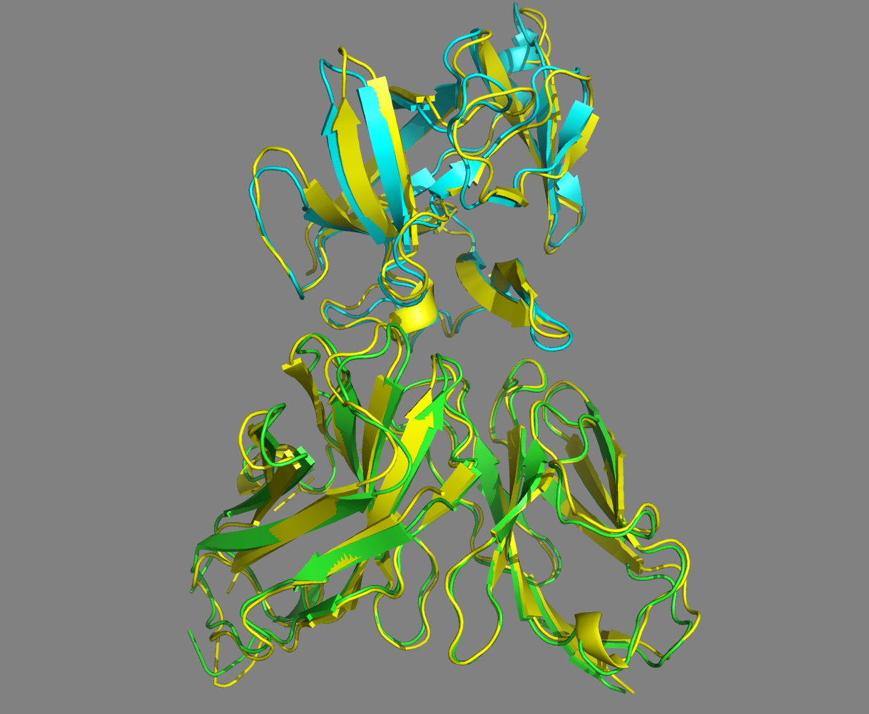
See the overlay of the top ranked model onto the reference structure expand_more
Top-ranked model of the top cluster (cluster1_model_1) superimposed onto the reference crystal structure (in yellow)
Conclusions
We have demonstrated the usage of HADDOCK3 in an antibody-antigen docking scenario making use of the paratope information on the antibody side (i.e. no prior experimental information, but computational predictions) and an NMR-mapped epitope for the antigen. Compared to the static HADDOCK2.X workflow, the modularity and flexibility of HADDOCK3 allow to customise the docking protocols and to run a deeper analysis of the results. HADDOCK3’s intrinsic flexibility can be used to improve the performance of antibody-antigen modelling compared to the results we presented in our Structure 2020 article and in the related HADDOCK2.4 tutorial.
BONUS 1: Dissecting the interface energetics: what is the impact of a single mutation?
Mutations at the binding interfaces can have widely varying effects on binding affinity - some may be negligible, while others can significantly strengthen or weaken the interaction. Exploring these mutations helps identify critical amino acids for redesigning structurally characterized protein-protein interfaces, which paves the way for developing protein-based therapeutics to deal with a diverse range of diseases. To pinpoint such amino acids positions, the residues across the protein interaction surfaces are either randomly or strategically mutated. Scanning mutations in this manner is experimentally costly. Therefore, computational methods have been developed to estimate the impact of an interfacial mutation on protein-protein interactions. These computational methods come in two main flavours. One involves rigorous free energy calculations, and, while highly accurate, these methods are computationally expensive. The other category includes faster, approximate approaches that predict changes in binding energy using statistical potentials, machine learning, empirical scoring functions etc. Though less precise, these faster methods are practical for large-scale screening and early-stage analysis. In this bonus exercise, we will take a look at two quick ways of estimating the effect of a single mutation in the interface.
PROT-ON and haddock3-scoring to inspect a single mutation
PROT-ON (Structure-based detection of designer mutations in PROTein-protein interface mutatiONs) is a tool and online server that scans all possible interfacial mutations and predicts ΔΔG score by using EvoEF1 (active in both on the web server and stand-alone versions) or FoldX (active only in the stand-alone version) with the aim of finding the most mutable positions. The original publication describing PROT-ON can be found here.
Here we will use PROT-ON to analyse the interface of our antibody-antigen complex. For that, we will use the provided matched reference structure (4G6M-matched.pdb) in which both chains of the antibody have the same chainID (A), which allows us to analyse all interface residues of the antibody at once.
Note: Pre-calculated PROT-ON results for this system can be accessed here.
Connect to the PROT-ON server page (link above) and fill in the following fields:
Specify your run name* –> 4G6M_matched
Choose / Upload your protein complex* –> Select the provided 4G6M-matched.pdb file
Which dimer chains should be analyzed* –> Select chain A for the 1st molecule and B for the 2nd Pick the monomer for mutational scanning* –> Select the first molecule - the antibody (toggle the switch ON under the chain A)
Your run should complete in 5-10 minutes. Once finished, you will be presented with a result page summarising the most depleting (ones that decrease the binding affinity) and most enriching (ones that increase the binding affinity) mutations.
Which possible mutation would you propose to improve the binding affinity of the antibody?
See answer expand_more
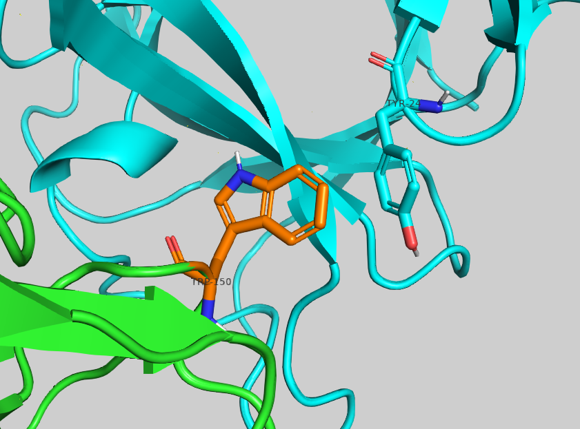
The most enriching mutation is S150W with a -3.69 ΔΔG score.Inspect the proposed amino acid in PyMol. Can you rationalise why it might increase the affinity?
With HADDOCK3, it is possible to take a step further. To perform the mutation, simply rename the desired residue and score such model - HADDOCK will take care of the topology regardless of the side chain differences and energy minimisation of the model. To do so, first either edit 4G6M-matched.pdb in your favourite text editor and save this new file as 4G6M_matched_S150W.pdb, or use the command line: sed ‘s/SER\ A\ 150/TRP\ A\ 150/g’ 4G6M_matched.pdb > 4G6M_matched_S150W.pdb
Next, score the mutant using the command-line tool haddock3-score.
This tool performs a short workflow composed of the topoaa and emscoring modules. Use flag --outputpdb to save energy-minimized model:
haddock3-score 4G6M_matched_S150W.pdb --outputpdb
Zoom in on the mutated residue expand_more
Alanine Scanning module
Another way of exploring interface energetics is by using the alascan module of HADDOCK3. alascan stands for “Alanine Scanning module”.
This module is capable of mutating interface residues to Alanine and calculating the Δ HADDOCK score between the wild-type and mutant, thus providing a measure of the impact of each individual mutation. It is possible to scan all interface residues one by one or limit this scanning to a selected by user set of residues. By default, the mutation to Alanine is performed, as its side chain is just a methyl group, so side chain perturbations are minimal, as well as possible secondary structure changes. It is possible to perform the mutation to any other amino acid type - at your own risk, as such mutations may introduce structural uncertainty.
Important: 1/ alascan calculates the difference between wild-type score vs mutant score, i.e. positive Δscore indicative of the enriched (stronger) binding and negative Δscore is indicative of the depleted (weaker) binding; 2/ Inside alascan, a short energy minimization of an input structure is performed, i.e. there’s no need to include an additional refinement module prior to alascan.
Here is an example of the workflow to scan interface energetics:
# ====================================================================
# Scanning interface residues with haddock3
# ====================================================================

# directory in which the scoring will be done
run_dir = "run-energetics-alascan"

# compute mode
mode = "local"
ncores = 50

# Post-processing to generate statistics and plots
postprocess = true
clean = true

molecules =  [
    "pdbs/4G6M_matched.pdb",
    ]

# ====================================================================
# Parameters for each stage are defined below
# ====================================================================
[topoaa]

[alascan]
# mutate each interface residue to Alanine
scan_residue = 'ALA'
# generate plot of delta score and its components per each mutation
plot = true

# ====================================================================
A scoring scenario configuration file is provided in the workflows/ directory as interaction-energetics.cfg, and precomputed results are in runs/run-energetics-alascan.
The output folder contains, among others, a directory titled 1_alascan with a file scan_4G6M_matched_haddock.tsv that lists each mutation, corresponding score and individual terms:
################################################################################
# `alascan` results for 4G6M_matched_haddock
#
# native score = -147.0143
#
# z_score is calculated with respect to the other residues
################################################################################
chain   res     ori_resname     end_resname     score   vdw     elec    desolv  bsa     delta_score     delta_vdw       delta_elec      delta_desolv      delta_bsa       z_score
A       32      SER     ALA     -147.00 -64.67  -446.68  7.01    1687.98  -0.01  -0.44   -0.14   0.46    6.61    0.81
A       33      GLY     ALA     -145.44 -64.53  -447.10  8.50    1685.78  -1.57  -0.59    0.27  -1.04    8.81    0.59
A       54      TRP     ALA     -142.68 -60.57  -450.75  8.04    1693.72  -4.33  -4.55    3.92  -0.57    0.87    0.18
A       55      TRP     ALA     -137.40 -60.24  -445.77 12.00    1654.06  -9.61  -4.87   -1.06  -4.53   40.53   -0.59
A       56      ASP     ALA     -132.71 -65.76  -360.08  5.07    1685.35 -14.30   0.65  -86.75   2.40    9.24   -1.27
A       58      ASP     ALA     -123.54 -62.33  -325.03  3.79    1648.48 -23.47  -2.78 -121.80   3.67   46.11   -2.61
A       59      GLU     ALA     -147.22 -65.46  -444.85  7.21    1692.34   0.21   0.35   -1.98   0.25    2.25    0.85
A       60      SER     ALA     -145.33 -65.48  -435.30  7.21    1700.59  -1.69   0.37  -11.53   0.25   -6.00    0.57
...
You can use an additional script /scripts/get-alascan-extrema.sh to check your answer:
bash scripts/get-alascan-extrema.sh run-energetics-alascan/1_alascan/scan_4G6M_matched_haddock.tsv
Mutation of the residue ASP58 turned out to be the most depleting within chain A. Let us visualise it in PyMol to analyse its contribution to the binding: File menu -> Open -> 4G6M_matched.pdb
Display ASP58 as sticks and colour it by atom:
util.cbc
select asp58, (resi 58 and chain A)
show sticks, asp58
util.cbao asp58
Now visualise its neighbouring residues:
select asp58_neighbour_atoms_4A, (resi 58 and chain A) around 4 and chain B
select asp58_neighbour_residues, byres asp58_neighbour_atoms_4A
show sticks, asp58_neighbour_residues
util.cbao asp58_neighbour_residues
Let us display contacts using show contacts plugin:
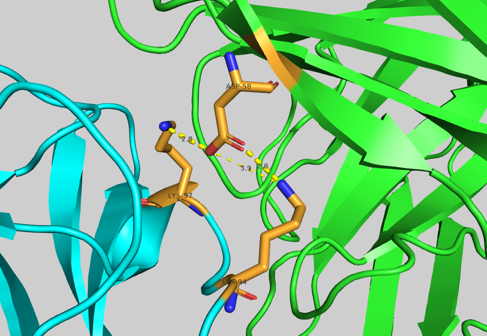
We can see one hydrogen bond between ASP58 and LYS98, and two hydrogen bonds ASP58 and LYS94.
Mutating ASP58 to ALA should result in the disappearance of those h-bonds, and the overall depletion of the binding.
This is reflected by the high negative value (-136.01) of delta_elec in either of .tsv files.
Let us test several mutations to confirm our hypothesis. Here is an example of the workflow to perform such mutations and save generated models:
# ====================================================================
# Mutating selected interface residue with haddock3
# ====================================================================

# directory in which the scoring will be done
run_dir = "run-energetics-mutations"

# compute mode
mode = "local"
ncores = 50

# Post-processing to generate statistics and plots
postprocess = true
clean = true

molecules =  ["pdbs/4G6M_matched.pdb"]

# ====================================================================
# Parameters for each stage are defined below
# ====================================================================
[topoaa]

[alascan]
# mutate residue 58 of chain A to Arginine
scan_residue = "ARG"
resdic_A = [58]
# save energy-minimised mutant model
output_mutants= true

[alascan]
scan_residue = "GLY"
resdic_A = [58]
output_mutants= true

[alascan]
scan_residue = "TRP"
resdic_A = [58]
output_mutants= true
Configuration file for this scenario can be found in workflows/single-residue-mutations.cfg, precomputed results are in run-residue-mutations. The output folder contains, among others, an energy-minimised mutant model 1_alascan/4G6M_matched_haddock-A_D58R.pdb.gz, and tables .tsv with energetics.
Take a look at the scores of the mutants. Which mutation depletes binding the most?
Inspect the mutant vs wild-type complex. Can you see the difference at the interface level?
See the overlay of the mutant onto the wild-type structure expand_more
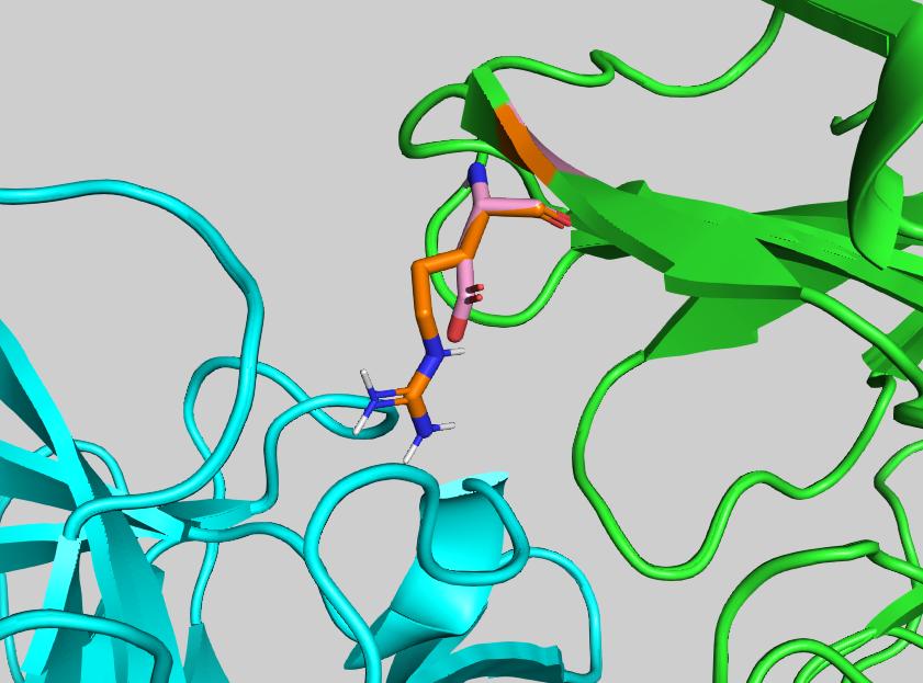
See answer expand_more
The values themselves are expected to differ, because [alascan] calculates ΔHADDOCK score, while PROT-ON predicts ΔΔG. Moreover, both tools are making predictions using different methods, so it is normal to have different results. However, if both tools consistently identify the same mutations as binding enriching or depleting - this may signal that selected residues indeed play a key role in binding affinity.Now let us consider how sensitive this kind of analysis is to the quality of the docking model. Instead of using the crystal structure, repeat this analysis using the best model of the top-ranked cluster or the best model with the lowest LRMSD value.
BONUS 2: Does the antibody bind to a known interface of interleukin? ARCTIC-3D analysis
Gevokizumab is a highly specific antibody that targets an allosteric site of Interleukin-1β (IL-1β) in PDB file 4G6M, thus reducing its binding affinity for its substrate, interleukin-1 receptor type I (IL-1RI). Canakinumab, another antibody binding to IL-1β, has a different mode of action, as it competes directly with the binding site of IL-1RI (in PDB file 4G6J). For more details please check this article.
We will now use our new software, ARCTIC-3D, to visualize the binding interfaces formed by IL-1β. First, the program retrieves all the existing binding surfaces formed by IL-1β from the PDBe website. Then, these binding surfaces are compared and clustered together if they span a similar region of the selected protein (IL-1β in our case).
We will run an ARCTIC-3D job targeting the uniprot ID of human Interleukin-1 beta, namely P01584.
For this first open the ARCTIC-3D web-server page here.
Insert the selected UniProt ID in the UniprotID field.
Leave the other parameters as they are and click on Submit.
Wait a few seconds for the job to complete or access a precalculated run here.
How many interface clusters were found for this protein?
Once you download the output archive, you can find the clustering information presented in the dendrogram:
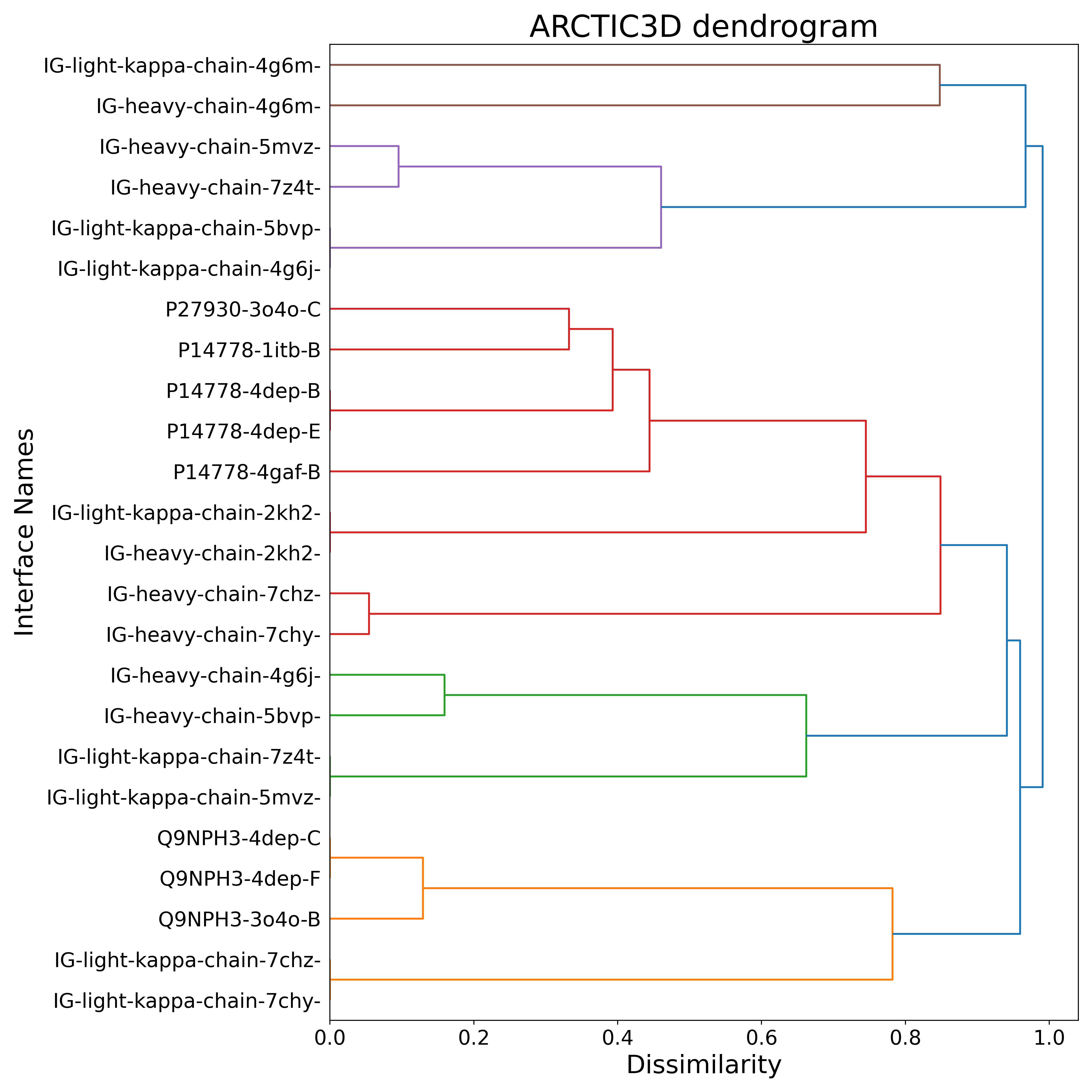
We can see how the two 4G6M antibody chains are recognized as a unique cluster, clearly separated from the other binding surfaces and, in particular, from those proper to IL-1RI (uniprot ID P14778).
Re-run ARCTIC-3D with a clustering threshold equal to 0.95
This means that the clustering will be looser, therefore lumping more dissimilar surfaces into the same object.
You can inspect a precalculated run here.
BONUS 3: How good are AI-based models of antibody for docking?
The release of AlphaFold2 in late 2020 has brought structure prediction methods to a new frontier, providing accurate models for the majority of known proteins. This revolution did not spare antibodies, with Alphafold2-multimer and other prediction methods (most notably ABodyBuilder2, from the ImmuneBuilder suite) performing nicely on the variable regions.
For a short introduction to AI and AlphaFold2 refer to this other tutorial introduction.
For antibody modelings, CDR loops are clearly the most challenging region to be predicted given their high sequence variability and flexibility. Multiple Sequence Alignment (MSA)-derived information is also less useful in this context.
Here we will see whether the antibody models given by Alphafold2-multimer and ABodyBuilder2 can be used for generating reliable models of the antibody-antigen complex by docking, instead of the unbound form used in this tutorial, which, in many cases, will not be available.
Analysing the AI models
We already ran the prediction with these two tools, and you can find the resulting models in the pdbs directory as:
4g6k_Abodybuilder2.pdb4g6k_AF2_multimer.pdb
As was demonstrated in the tutorial, those files must be preprocessed for their use in HADDOCK. Docking-ready files are also provided in the pdbs directory:
4G6K_abb_clean.pdb4G6K_af2_clean.pdb
Load the experimental unbound structure (4G6K_clean.pdb) and the two AI models in PyMOL to see whether they resemble the experimental unbound structure.
File menu -> Open -> select 4G6K_clean.pdb File menu -> Open -> select 4G6K_abb_clean.pdb File menu -> Open -> select 4G6K_af2_clean.pdb
Align the models to the experimental unbound structure
Which model is the closest to the unbound conformation?
See the RMSD values expand_more
  4G6K_abb_clean       RMSD =    0.428 Å
  4G6K_af2_clean       RMSD =    0.765 Å
For docking purposes however, it might be more interesting to know how far are the models from the bound conformation, i.e. the conformation in the antibody-antigen complex. The closer it is, the easier it should become to model the complex by docking. To assess this, we can load the structure of the complex in PyMOL and align all other structures/models to it.
File menu -> Open -> select 4G6M_matched.pdb
Align now the models to the experimental bound structure
alignto 4G6M_matched and chain A
Which model is the closest to the bound conformation?
See the RMSD values expand_more
  4G6K_abb_clean       RMSD =    0.330 Å
  4G6K_af2_clean       RMSD =    0.675 Å
  4G6K_clean           RMSD =    0.393 Å
Docking performance using AI-based antibody models
We can repeat the docking as described above in our tutorial, but using this time either the ABodyBuilder2 or AlphaFold2 models as input.
For this, modify your haddock3 configuration file, changing the input PDB file of the first molecule (the antibody) using the respective HADDOCK-ready models provided in the pdbs directory.
You will also need to change the restraint filename used to keep the two parts of the antibody together (those files are present in the restraints directory.
Further, run haddock3 as described above.
Pre-calculated runs are provided in the runs directory. Analyse your run (or the pre-calculated ones) as described previously.
See the cluster statistics expand_more
==============================================
== run1/10_caprieval/capri_clt.tsv
==============================================
Total number of acceptable or better clusters:  1  out of  4
Total number of medium or better clusters:      1  out of  4
Total number of high quality clusters:          1  out of  4

First acceptable cluster - rank:  1  i-RMSD:  0.997  Fnat:  0.853  DockQ:  0.830
First medium cluster     - rank:  1  i-RMSD:  0.997  Fnat:  0.853  DockQ:  0.830
Best cluster             - rank:  1  i-RMSD:  0.997  Fnat:  0.853  DockQ:  0.830

==============================================
== run1-abb/10_caprieval/capri_clt.tsv
==============================================
Total number of acceptable or better clusters:  1  out of  4
Total number of medium or better clusters:      1  out of  4
Total number of high quality clusters:          0  out of  4

First acceptable cluster - rank:  1  i-RMSD:  1.122  Fnat:  0.832  DockQ:  0.802
First medium cluster     - rank:  1  i-RMSD:  1.122  Fnat:  0.832  DockQ:  0.802
Best cluster             - rank:  1  i-RMSD:  1.122  Fnat:  0.832  DockQ:  0.802

==============================================
== run1-af2//10_caprieval/capri_clt.tsv
==============================================
Total number of acceptable or better clusters:  3  out of  3
Total number of medium or better clusters:      0  out of  3
Total number of high quality clusters:          0  out of  3

First acceptable cluster - rank:  1  i-RMSD:  2.728  Fnat:  0.440  DockQ:  0.457
Best cluster             - rank:  1  i-RMSD:  2.728  Fnat:  0.440  DockQ:  0.457
Which starting structure of the antibody gives the best overall model (irrespective of the ranking)?
Hint: Use the extract-capri-stats.sh script to analyse the various runs and find the best (lowest i-RMSD or highest Dock-Q score) as the emref stage.
See single structure statistics expand_more
==============================================
== run1/07_caprieval/capri_ss.tsv
==============================================
...
First acceptable model - rank:  1  i-RMSD:  1.287  Fnat:  0.759  DockQ:  0.741
First medium model     - rank:  1  i-RMSD:  1.287  Fnat:  0.759  DockQ:  0.741
Best model             - rank:  2  i-RMSD:  0.805  Fnat:  0.931  DockQ:  0.894

==============================================
== run1-abb/07_caprieval/capri_ss.tsv
==============================================
...
First acceptable model - rank:  1  i-RMSD:  1.230  Fnat:  0.845  DockQ:  0.795
First medium model     - rank:  1  i-RMSD:  1.230  Fnat:  0.845  DockQ:  0.795
Best model             - rank:  5  i-RMSD:  0.919  Fnat:  0.845  DockQ:  0.843

==============================================
== run1-af2/07_caprieval/capri_ss.tsv
==============================================
...
First acceptable model - rank:   1  i-RMSD:  2.928  Fnat:  0.431  DockQ:  0.390
First medium model     - rank:  11  i-RMSD:  1.599  Fnat:  0.569  DockQ:  0.613
Best model             - rank:  16  i-RMSD:  1.451  Fnat:  0.621  DockQ:  0.674
Conclusions - AI-based docking
All three antibody structures used in input give good to reasonable results. The unbound and the ABodyBuilder2 antibodies provided better results, with the best cluster showing models within 1 angstrom of interface-RMSD with respect to the unbound structure. Using the Alphafold2 structure in this case is not the best option, as the input antibody is not perfectly modelled in its H3 loop.
BONUS 4: Ensemble docking using a combination of exprimental and AI-predicted antibody structures
Instead of running haddock3 using a specific input structure of the antibody, we can also use an ensemble of all available models.
Such an ensemble can be created from the individual models using pdb_mkensemble from PDB-tools:
pdb_mkensemble 4G6K_clean.pdb 4G6K_abb_clean.pdb 4G6K_af2_clean.pdb > 4G6K-ensemble.pdb
This ensemble file is provided in the pdbs directory.
Now we can make use of the flexibility of haddock3 in defining workflows to add a clustering step after the rigid body docking step in order to make sure that models originating from all models will ideally be selected for the refinement steps (provided they do cluster). This modified workflow looks like:
# ====================================================================
# Antibody-antigen docking example with restraints from the antibody
# paratope to the NMR-identified epitope on the antigen
# ====================================================================

# directory in which the scoring will be done
run_dir = "run-ens-CDR-NMR-CSP"

# compute mode
mode = "local"
ncores = 50

# Post-processing to generate statistics and plots
postprocess = true
clean = true

molecules =  [
    "pdbs/4G6K-ensemble.pdb",
    "pdbs/4I1B_clean.pdb"
    ]

# ====================================================================
# Parameters for each stage are defined below, prefer full paths
# ====================================================================
[topoaa]

[rigidbody]
# CDR to NMR epitope ambig restraints
ambig_fname = "restraints/ambig-paratope-NMR-epitope.tbl"
# Restraints to keep the antibody chains together
unambig_fname = "restraints/antibody-unambig.tbl"
# Reduced sampling (150 instead of the default of 1000)
# Increased to 150 so that each conformation is sampled 50 times
sampling = 150

[caprieval]
reference_fname = "pdbs/4G6M_matched.pdb"

[clustfcc]
plot_matrix = true

[seletopclusts]
top_models = 10

[caprieval]
reference_fname = "pdbs/4G6M_matched.pdb"

[flexref]
tolerance = 5
# CDR to NMR epitope ambig restraints
ambig_fname = "restraints/ambig-paratope-NMR-epitope.tbl"
# Restraints to keep the antibody chains together
unambig_fname = "restraints/antibody-unambig.tbl"

[caprieval]
reference_fname = "pdbs/4G6M_matched.pdb"

[emref]
tolerance = 5
# CDR to NMR epitope ambig restraints
ambig_fname = "restraints/ambig-paratope-NMR-epitope.tbl"
# Restraints to keep the antibody chains together
unambig_fname = "restraints/antibody-unambig.tbl"

[caprieval]
reference_fname = "pdbs/4G6M_matched.pdb"

[clustfcc]
plot_matrix = true

[seletopclusts]
top_models = 4

[caprieval]
reference_fname = "pdbs/4G6M_matched.pdb"

[contactmap]

# ====================================================================
Our workflow consists of the following 14 modules:
topoaa: Generates the topologies for the CNS engine and builds missing atomsrigidbody: Performs Rigid body energy minimisation - with increased sampling (150 models - 50 per input model)caprieval: Calculates CAPRI metricsclustfcc: Clustering of models based on the fraction of common contacts (FCC)seletopclusts: Selects the top models of all clusters - In this case, we select max 10 models per cluster.caprieval: Calculates CAPRI metrics of the selected clustersflexref: Performs Semi-flexible refinement of the interface (it1in haddock2.4)caprievalemref: Performs a final refinement by energy minimisation (itwEM only in haddock2.4)caprievalclustfcc: Clustering of models based on the fraction of common contacts (FCC)seletopclusts: Selects the top models of all clusterscaprievalcontactmap: Contacts matrix and a chordchart of intermolecular contacts
Compared to the original workflow described in this tutorial we have added clustering and cluster selections steps after the rigid body docking.
Run haddock3 with this configuration file as described above.
A pre-calculated run is provided in the runs directory as run1-ens.
Analyse your run (or the pre-calculated ones) as described previously.
See the cluster statistics expand_more
==============================================
== run1-ens//12_caprieval/capri_clt.tsv
==============================================
Total number of acceptable or better clusters:  3  out of  12
Total number of medium or better clusters:      1  out of  12
Total number of high quality clusters:          1  out of  12

First acceptable cluster - rank:  1  i-RMSD:  0.973  Fnat:  0.875  DockQ:  0.836
First medium cluster     - rank:  1  i-RMSD:  0.973  Fnat:  0.875  DockQ:  0.836
Best cluster             - rank:  1  i-RMSD:  0.973  Fnat:  0.875  DockQ:  0.836
See single structure statistics expand_more
==============================================
== run1-ens//02_caprieval/capri_clt.tsv
==============================================
Total number of acceptable or better clusters:  0  out of  1
Total number of medium or better clusters:      0  out of  1
Total number of high quality clusters:          0  out of  1

First acceptable cluster - rank:   i-RMSD:   Fnat:   DockQ:
First medium cluster     - rank:   i-RMSD:   Fnat:   DockQ:
Best cluster             - rank:  -  i-RMSD:  14.309  Fnat:  0.056  DockQ:  0.060
==============================================
== run1-ens//05_caprieval/capri_clt.tsv
==============================================
Total number of acceptable or better clusters:  3  out of  12
Total number of medium or better clusters:      1  out of  12
Total number of high quality clusters:          0  out of  12

First acceptable cluster - rank:  2  i-RMSD:  1.305  Fnat:  0.651  DockQ:  0.682
First medium cluster     - rank:  2  i-RMSD:  1.305  Fnat:  0.651  DockQ:  0.682
Best cluster             - rank:  2  i-RMSD:  1.305  Fnat:  0.651  DockQ:  0.682
==============================================
== run1-ens//07_caprieval/capri_clt.tsv
==============================================
Total number of acceptable or better clusters:  0  out of  1
Total number of medium or better clusters:      0  out of  1
Total number of high quality clusters:          0  out of  1

First acceptable cluster - rank:   i-RMSD:   Fnat:   DockQ:
First medium cluster     - rank:   i-RMSD:   Fnat:   DockQ:
Best cluster             - rank:  -  i-RMSD:  7.663  Fnat:  0.172  DockQ:  0.136
==============================================
== run1-ens//09_caprieval/capri_clt.tsv
==============================================
Total number of acceptable or better clusters:  0  out of  1
Total number of medium or better clusters:      0  out of  1
Total number of high quality clusters:          0  out of  1

First acceptable cluster - rank:   i-RMSD:   Fnat:   DockQ:
First medium cluster     - rank:   i-RMSD:   Fnat:   DockQ:
Best cluster             - rank:  -  i-RMSD:  7.619  Fnat:  0.164  DockQ:  0.133
==============================================
== run1-ens//12_caprieval/capri_clt.tsv
==============================================
Total number of acceptable or better clusters:  3  out of  12
Total number of medium or better clusters:      1  out of  12
Total number of high quality clusters:          1  out of  12

First acceptable cluster - rank:  1  i-RMSD:  0.973  Fnat:  0.875  DockQ:  0.836
First medium cluster     - rank:  1  i-RMSD:  0.973  Fnat:  0.875  DockQ:  0.836
Best cluster             - rank:  1  i-RMSD:  0.973  Fnat:  0.875  DockQ:  0.836
We started from three different conformations of the antibody: 1) the unbound crystal structure, 2) the ABodyBuilder2 model and 3) the AlphaFold2 model.
BONUS 5: Antibody-antigen complex structure prediction from sequence using AlphaFold2
With the advent of Artificial Intelligence (AI) and AlphaFold2, we can also try to predict directly the full antibody-antigen complex using AlphaFold2. For this we are going to use the AlphaFold2_mmseq2 Jupyter notebook which can be found with other interesting notebooks in Sergey Ovchinnikov ColabFold GitHub repository, making use of the Google Colab CLOUD resources.
Start the AlphaFold2 notebook on Colab by clicking here.
Note: The bottom part of the notebook contains instructions on how to use it.
Setting up the antibody-antigen complex prediction with AlphaFold2
To setup the prediction we need to provide the sequence of the heavy and light chains of the antibody and the sequence of the antigen. These are respectively
- Antibody heavy chain:
QVQLQESGPGLVKPSQTLSLTCSFSGFSLSTSGMGVGWIRQPSGKGLEWLAHIWWDGDES
YNPSLKSRLTISKDTSKNQVSLKITSVTAADTAVYFCARNRYDPPWFVDWGQGTLVTVSS
- Antibody light chain:
DIQMTQSTSSLSASVGDRVTITCRASQDISNYLSWYQQKPGKAVKLLIYYTSKLHSGVPS
RFSGSGSGTDYTLTISSLQQEDFATYFCLQGKMLPWTFGQGTKLEIK
- Antigen:
VRSLNCTLRDSQQKSLVMSGPYELKALHLQGQDMEQQVVFSMSFVQGEESNDKIPVALGL
KEKNLYLSCVLKDDKPTLQLESVDPKNYPKKKMEKRFVFNKIEINNKLEFESAQFPNWYI
STSQAENMPVFLGGTKGGQDITDFTMQFVSS
To use AlphaFold2 to predict this antibody-antigen complex follow the following steps:
For your convenience the full sequence with colons is provided:
QVQLQESGPGLVKPSQTLSLTCSFSGFSLSTSGMGVGWIRQPSGKGLEWLAHIWWDGDESYNPSLKSRLTISKDTSKNQVSLKITSVTAADTAVYFCARNRYDPPWFVDWGQGTLVTVSS:DIQMTQSTSSLSASVGDRVTITCRASQDISNYLSWYQQKPGKAVKLLIYYTSKLHSGVPSRFSGSGSGTDYTLTISSLQQEDFATYFCLQGKMLPWTFGQGTKLEIK:VRSLNCTLRDSQQKSLVMSGPYELKALHLQGQDMEQQVVFSMSFVQGEESNDKIPVALGLKEKNLYLSCVLKDDKPTLQLESVDPKNYPKKKMEKRFVFNKIEINNKLEFESAQFPNWYISTSQAENMPVFLGGTKGGQDITDFTMQFVSS
Define the jobname, e.g. Ab-Ag
In the top section of the Colab, click: Runtime > Run All
(It may give a warning that this is not authored by Google because it is pulling code from GitHub - you can ignore it).
This will automatically install, configure and run AlphaFold2 for you - leave this window open. After the prediction completed, you will be asked to download a zip archive with the results (if you configured it to use Google Drive, a result archive will be automatically saved to your Google Drive).
Time to grab a cup of tea or a coffee!
And while waiting try to answer the following questions:
How do you interpret AlphaFold2 predictions? What are the predicted LDDT (pLDDT), PAE, iptm?
Tip: Try to find information about the prediction confidence at https://alphafold.ebi.ac.uk/faq. A nice summary can also be found here.
Pre-calculated AlphFold2 predictions are provided here. This archive contains the five predicted models (the naming indicates the rank), figures (png) files (PAE, pLDDT, coverage) and json files containing the corresponding values (the last part of the json files report the ptm and iptm values).
Analysis of the generated AF2 models
While the notebook is running, models will appear first under the Run Prediction section, colored both by chain and by pLDDT.
The best model will then be displayed under the Display 3D structure section. This is an interactive 3D viewer that allows you to rotate the molecule and zoom in or out.
Note that you can change the model displayed with the rank_num option. After changing, it execute the cell by clicking on the run cell icon on the left of it.
How similar are the five models generated by AF2?
Consider the pLDDT of the various models (the higher the pLDDT the more reliable the model).
While the pLDDT score is an overall measure, you can also focus on the interface score reported in the iptm score (value between 0 and 1).
See the confidence statistics for the five generated models
    Model1: pLDDT=90.4 pTM=0.654 ipTM=0.525
    Model2: pLDDT=88.0 pTM=0.65  ipTM=0.522
    Model3: pLDDT=88.2 pTM=0.647 ipTM=0.52
    Model4: pLDDT=88.0 pTM=0.644 ipTM=0.516
    Model5: pLDDT=88.1 pTM=0.641 ipTM=0.512
Note that if you performed a fresh run your results might well differ from those shown here.
Based on the iptm scores, would you qualify those models as reliable?
Note that in this case the iptm score reports on all interfaces, i.e. both the interface between the two chains of the antibody, and the antibody-antigen interface
Another useful way of looking at the model accuracy is to check the Predicted Alignment Error plots (PAE) (also referred to as Domain position confidence). The PAE gives a distance error for every pair of residues: It gives the estimate of the position error at residue x when the predicted and true structures are aligned on residue y. Values range from 0 to 35 Angstroms. It is usually shown as a heatmap image with residue numbers running along vertical and horizontal axes and each pixel colored according to the PAE value for the corresponding pair of residues. If the relative position of two domains is confidently predicted then the PAE values will be low (less than 5A - dark blue) for pairs of residues with one residue in each domain. When analysing your complex, the diagonal block will indicate the PAE within each molecule/domain, while the off-diagonal blocks report the accuracy of the domain-domain placement.
Our antibody-antigen complex consists of three interfaces:
- The interface between the heavy and light chains of the antibody
- The interface between the heavy chain of the antibody and the antigen
- The interface between the light chain of the antibody and the antigen
See the PAE plots for the five generated models
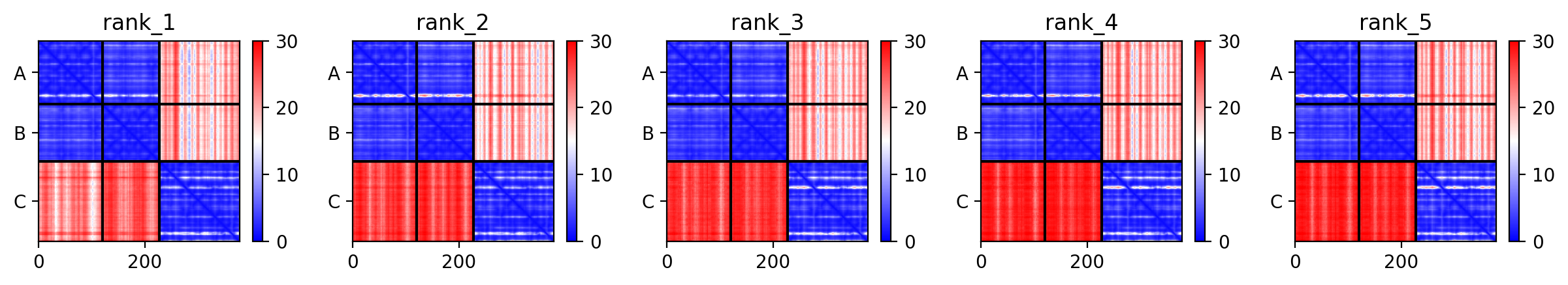
Based on the PAE plots, which interfaces can be considered reliable/unreliable?
Visualization of the generated AF2 models
In order to visualize the models in PyMOL save your predictions to disk or download the precalculated AlphaFold2 models from here.
Start PyMOL and load via the File menu all five AF2 models.
Repeat this for each model (abagtest_2d03e_unrelaxed_rank_X_alphafold2_multimer_v3_model_X_seed_000.pdb or whatever the naming of your model is).
Let us superimpose all models on the antibody (the antibody in the provided AF2 models correspond to chains A and B):
This will align all clusters on the antibody, maximizing the differences in the orientation of the antigen.
Examine the various models. How does the orientation of the antigen differ between them?
Note: You can turn on and off a model by clicking on its name in the right panel of the PyMOL window.
See tips on how to visualize the prediction confidence in PyMOL
When looking at the structures generated by AlphaFold2 in PyMOL, the pLDDT is encoded as the B-factor.To color the model according to the pLDDT type in PyMOL:
spectrum b **Note** that the scale in the B-factor field is the inverse of the color coding in the PAE plots: i.e. red mean reliable (high pLDDT) and blue unreliable (low pLDDT))
Since we do have NMR chemical shift perturbation data for the antigen, we can check if the perturbed residues are at the interface in the AF2 models. Note that there is a shift in the numbering of 2 residues between the AF2 and the HADDOCK models.
Does any model have the NMR-identified epitope at the interface with the antibody?
See the AlphaFold2 models with the NMR-mapped epitope
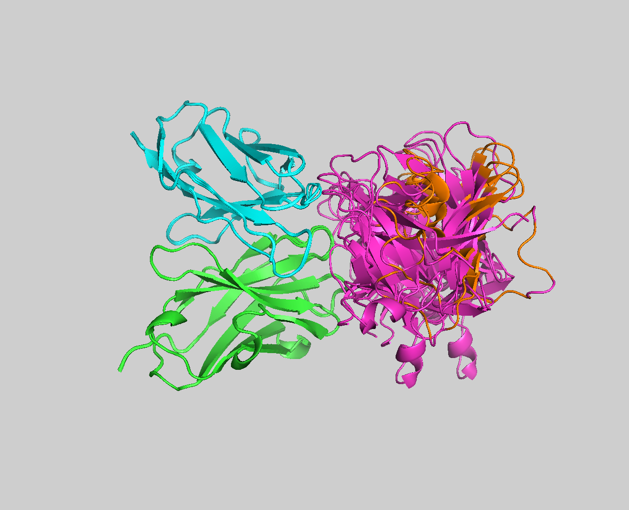
It should be clear from the visualization of the NMR-mapped epitope on the AF2 models that none satisfies the NMR data. To further make that clear we can compare the models to the crystal structure of the complex (4G6M).
For this download and superimpose the models onto the crystal structure in PyMOL with the following commands:
fetch 4G6M
remove resn HOH
color yellow, 4G6M
select 4G6M and chain H+L
alignto sele
See the AlphaFold2 models superimposed onto the crystal structure of the complex (4G6M)
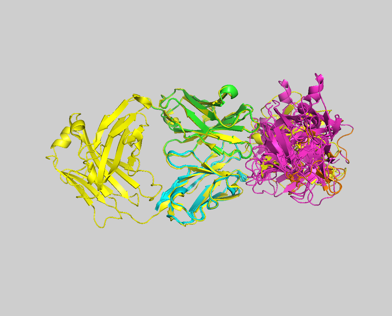
More recently, the third version of AlphaFold (AlphaFold3) has been published. While the code is not yet released, a dedicated online tool AlphaFoldServer is made available for the academic community to allow us to make upto 20 predictions per day with this new version. Pre-calculated AlphFold3 predictions are provided here.
See the AlphaFold3 models with mapped epitope residues in orange
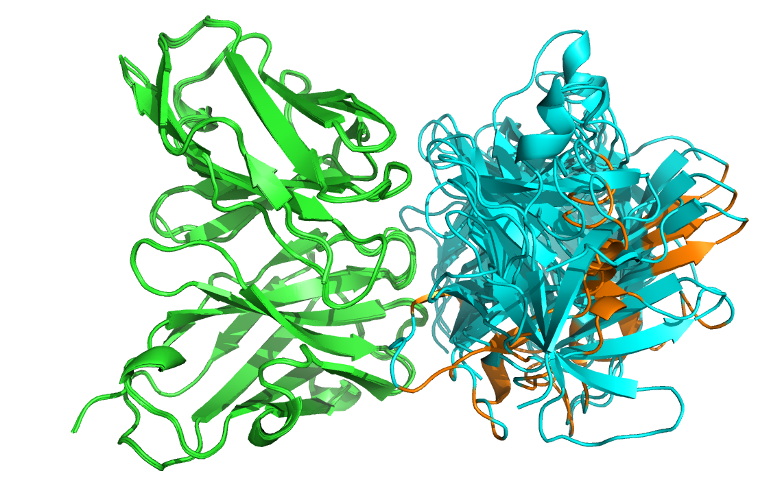
See the AlphaFold3 models onto the crystal structure of the complex (4G6M) in red
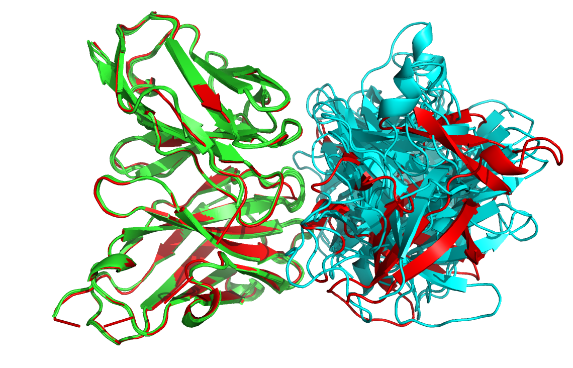
BONUS 6: Running a scoring scenario
This section demonstrates the use of HADDOCK3 to score the various models obtained at the previous stages (ensemble docking and AlphaFold predictions) and observe if the HADDOCK scoring function is able to detect the quality of the models.
To this end the following workflow is defined:
- Generate the topologies for the various models.
- Energy Minimise all complexes.
- Cluster the models using Fraction of Common Contacts:
- set the parameter
min_populationto 1 so that all models, including singletons (models that do not cluster with any others), will be forwarded to the next steps. - set the parameter
plot_matrixto true to generate a matrix of the clusters for a visual representation.
- set the parameter
- Comparison of the models with the reference complex
4G6M_matched.pdbusing CAPRI criteria.
For this, two ensembles must be scored and one structure will be used as a reference. You can find them in the pdbs/ directory:
07_emref_and_top5af2_ensemble.pdb: An ensemble of models obtained from the ensemble run, combined with top5 AlphaFold2 predictions.af3server_15052024_top5ens.pdb: An ensemble of top5 AlphaFold3 predictions.4G6M_matched.pdb: The reference structure for quality assessments.
# ====================================================================
# Antibody-antigen docking example with restraints from the antibody
# paratope to the NMR-identified epitope on the antigen
# ====================================================================
run_dir = "run-scoring"

molecules =  [
    "pdbs/haddock3-ens-emref-ensemble.pdb",
    "pdbs/af2-models.pdb",
    "pdbs/af3-models.pdb",
    ]

# ====================================================================
# Parameters for each stage are defined below
# ====================================================================

[topoaa]

[emscoring]

[clustfcc]
# Reduce the min_population to define a cluster to 1 so that models
# that do not cluster with any other will define singlotons
min_population = 1
# Generate a matrix of the clusters
plot_matrix = true

[caprieval]
reference_fname = "4G6M_matched.pdb"

# ====================================================================
A scoring scenario configuration file is provided in the workflows/ directory as scoring-antibody-antigen.cfg, precomputed results in runs/run-scoring`.
You can again look at the capri_ss.tsv file in the 4_caprieval directory. It contains the energy minimised statistics:
              model   md5     caprieval_rank  score   irmsd   fnat    lrmsd   ilrmsd  dockq   rmsd    cluster_id      cluster_ranking model-cluster_ranking   air       angles  bonds   bsa     cdih    coup    dani    desolv  dihe    elec    improper        rdcs    rg      sym     total   vdw     vean    xpcs
../1_emscoring/emscoring_2.pdb  -       1       -160.102        0.881   0.948   1.948   1.355   0.881   0.991   2       1       1       0.000   268.528   52.526  1887.330        0.000   0.000   0.000   3.250   2054.660        -522.959        72.589  0.000   0.000   0.000   -581.720        -58.760   0.000   0.000
../1_emscoring/emscoring_82.pdb -       2       -159.982        0.910   0.897   2.204   1.457   0.855   1.017   2       1       2       0.000   271.239   54.742  2015.530        0.000   0.000   0.000   7.494   2064.870        -601.662        70.926  0.000   0.000   0.000   -648.806        -47.144   0.000   0.000
../1_emscoring/emscoring_37.pdb -       3       -144.761        13.625  0.069   22.589  21.764  0.068   13.882  5       2       1       0.000   274.769   53.961  1805.280        0.000   0.000   0.000   5.497   2050.960        -466.808        75.165  0.000   0.000   0.000   -523.705        -56.897   0.000   0.000
../1_emscoring/emscoring_40.pdb -       4       -143.163        1.087   0.897   1.864   1.758   0.835   1.144   2       1       3       0.000   274.318   53.058  1891.460        0.000   0.000   0.000   2.661   2044.540        -471.775        76.007  0.000   0.000   0.000   -523.244        -51.468   0.000   0.000
../1_emscoring/emscoring_64.pdb -       5       -140.767        1.053   0.897   3.039   1.957   0.818   1.294   2       1       4       0.000   262.234   51.794  1794.740        0.000   0.000   0.000   -1.953  2035.620        -429.827        70.465  0.000   0.000   0.000   -482.676        -52.849   0.000   0.000
...
The emscoring module renames all models, which makes it difficult to know what was the original model.
You can however trace back a model to its original file by looking into the traceback/traceback.tsv file:
00_topo1                                                  1_emscoring             1_emscoring_rank
emref_10_from_haddock3-ens-emref-ensemble_2_haddock.psf   emscoring_2.pdb         1
emref_9_from_haddock3-ens-emref-ensemble_83_haddock.psf   emscoring_82.pdb        2
emref_47_from_haddock3-ens-emref-ensemble_42_haddock.psf  emscoring_37.pdb        3
emref_5_from_haddock3-ens-emref-ensemble_45_haddock.psf   emscoring_40.pdb        4
emref_7_from_haddock3-ens-emref-ensemble_67_haddock.psf   emscoring_64.pdb        5
...
A simple way to extra this information is to use grep:
See the output of grep for the AlphaFold2 models
> grep abag traceback.tsv
abagtest_2d03e_unrelaxed_rank_001_alphafold2_multimer_v3_model_3_seed_000_from_af2-models_1_haddock.psf	emscoring_84.pdb	86
abagtest_2d03e_unrelaxed_rank_005_alphafold2_multimer_v3_model_2_seed_000_from_af2-models_5_haddock.psf	emscoring_88.pdb	90
abagtest_2d03e_unrelaxed_rank_004_alphafold2_multimer_v3_model_4_seed_000_from_af2-models_4_haddock.psf	emscoring_87.pdb	91
abagtest_2d03e_unrelaxed_rank_003_alphafold2_multimer_v3_model_1_seed_000_from_af2-models_3_haddock.psf	emscoring_86.pdb	92
abagtest_2d03e_unrelaxed_rank_002_alphafold2_multimer_v3_model_5_seed_000_from_af2-models_2_haddock.psf	emscoring_85.pdb	93
See the output of grep for the AlphaFold3 models
> grep af3server traceback.tsv
af3server_15052024_2_ready_from_af3-models_2_haddock.psf	emscoring_90.pdb	45
af3server_15052024_1_ready_from_af3-models_1_haddock.psf	emscoring_89.pdb	84
af3server_15052024_4_ready_from_af3-models_4_haddock.psf	emscoring_92.pdb	87
af3server_15052024_3_ready_from_af3-models_3_haddock.psf	emscoring_91.pdb	88
af3server_15052024_5_ready_from_af3-models_5_haddock.psf	emscoring_93.pdb	89
We have already seen in the previous section that none of the AlphaFold models were close to the real complex. This is however also the case for some of the HADDOCK models. Still the AlpaFold models score very badly, toward the end of the ranked list of models.
See the answer
The bottom eight models (the worst ranking ones) are all AlphaFold3/2 models. Looking at the componenents of the score (some were left out in the table below for simplicity) one can see that it is mainly the van der Waals energy that causes the high scores, which is indicative of clashes in the models.
model               md5 caprieval_rank  score    irmsd   fnat    lrmsd   ilrmsd  dockq   rmsd    bsa        desolv    elec      vdw vean    xpcs
...
../1_emscoring/emscoring_90.pdb	-	45	-103.350	13.230	0.000	25.191	21.785	0.038	13.629	-	-	-	0.000	532.712	82.344	1664.180	0.000	0.000	0.000	5.540	1870.300	-290.416	180.660	0.000	0.000	0.000	-341.222	-50.807	0.000	0.000
...
../1_emscoring/emscoring_89.pdb	-	84	-74.275	13.209	0.000	24.538	21.430	0.040	13.545	-	-	-	0.000	508.920	76.308	1418.880	0.000	0.000	0.000	-0.571	1841.540	-257.010	165.391	0.000	0.000	0.000	-279.312	-22.301	0.000	0.000
../1_emscoring/emscoring_84.pdb	-	86	-67.914	11.123	0.000	22.413	18.626	0.048	12.213	-	-	-	0.000	770.364	255.616	3535.520	0.000	0.000	0.000	-67.537	1877.380	-150.913	337.834	0.000	0.000	0.000	-121.107	29.806	0.000	0.000
../1_emscoring/emscoring_92.pdb	-	87	-63.263	11.426	0.000	22.104	21.035	0.049	11.048	-	-	-	0.000	515.279	82.456	1383.920	0.000	0.000	0.000	-9.924	1823.120	-88.656	161.981	0.000	0.000	0.000	-124.263	-35.607	0.000	0.000
../1_emscoring/emscoring_91.pdb	-	88	-50.990	13.665	0.000	23.793	22.150	0.042	13.796	-	-	-	0.000	527.034	85.093	1492.150	0.000	0.000	0.000	-8.962	1854.670	-167.236	177.341	0.000	0.000	0.000	-175.816	-8.581	0.000	0.000
../1_emscoring/emscoring_93.pdb	-	89	-46.871	6.644	0.000	10.617	11.333	0.146	6.455	-	-	-	0.000	578.041	93.545	1740.990	0.000	0.000	0.000	-8.906	1846.130	-35.623	211.309	0.000	0.000	0.000	-66.464	-30.841	0.000	0.000
../1_emscoring/emscoring_88.pdb	-	90	48.283	12.919	0.000	20.484	19.885	0.053	14.706	-	-	-	0.000	766.051	243.660	3914.250	0.000	0.000	0.000	-68.786	1881.260	-129.461	337.076	0.000	0.000	0.000	13.500	142.961	0.000	0.000
../1_emscoring/emscoring_87.pdb	-	91	180.468	12.447	0.000	22.153	19.299	0.048	14.160	-	-	-	0.000	1572.570	762.062	3639.430	0.000	0.000	0.000	-66.857	1874.120	-240.130	561.687	0.000	0.000	0.000	55.221	295.351	0.000	0.000
../1_emscoring/emscoring_86.pdb	-	92	240.307	12.572	0.000	21.662	19.799	0.049	14.187	-	-	-	0.000	946.547	447.473	3535.820	0.000	0.000	0.000	-69.380	1933.090	-154.703	492.276	0.000	0.000	0.000	185.924	340.628	0.000	0.000
../1_emscoring/emscoring_85.pdb	-	93	781.210	15.174	0.000	23.497	24.993	0.042	17.151	-	-	-	0.000	1249.820	692.831	3278.340	0.000	0.000	0.000	-61.261	1890.630	-86.026	1048.420	0.000	0.000	0.000	773.651	859.677	0.000	0.000
Hint 1: The HADDOCK score is calculated over all existing interfaces defined by different chainIDs.
Hint 2: Visualise two of the models with very different BSA values, color-coding the chains.
Congratulations! 🎉
You have completed this tutorial. If you have any questions or suggestions, feel free to contact us via email or asking a question through our support center.
And check also our education web page where you will find more tutorials!