Basic protein-DNA docking using local version of Haddock3
This tutorial consists of the following sections:
- Introduction
- Software and data setup
- Understanding the Ambiguous Interaction Restraints
- Preparation of PDB files for the docking (optional)
- Docking with Haddock3
- Analysis of the docking results
- Congratulations!
Introduction
This tutorial demonstrates how to setup a Haddock3 workflow dedicated to predict the 3D structure of protein-DNA (double-stranded DNA) complexes using pre-defined restraints, derived from the literature, and symmetry restraints. Here, we introduce the basic concepts of HADDOCK, suitable for tackling various typical protein-DNA docking challenges:
- basic preparation of the input PDB files;
- creation of the suitable Haddock3 workflow;
- basic analysis of the docking results.
Please note that we do not cover the processing of literature data into docking restraints; for more information, please refer to the advanced tutorial.
Computation within this tutorial should take 1.5 hours on 8 CPUs. The tutorial data, as well as precomputed results available here.
Tutorial test case
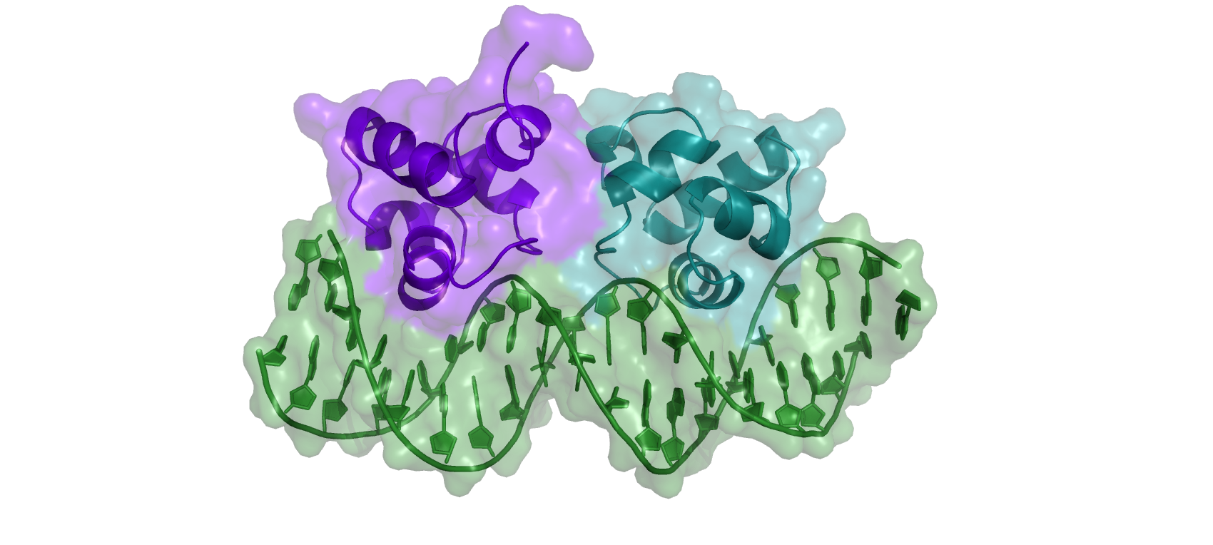
In this tutorial, we will work with the phage 434 Cro/OR1 complex (PDB: 3CRO), formed by bacteriophage 434 Cro repressor proteins and the OR1 operator.
Cro is part of the bacteriophage 434 genetic switch, playing a key role in controlling the switch between the lysogenic and lytic cycles of the bacteriophage. It is a repressor protein that works in opposition to the phage repressor cI protein to control the genetic switch. Both repressors compete to gain control over an operator region containing three operators that determine the state of the lytic/lysogenic genetic switch. If Cro prevails, the late genes of the phage will be expressed, resulting in lysis. Conversely, if the cI repressor prevails, the transcription of Cro genes is blocked, and cI repressor synthesis is maintained, resulting in a state of lysogeny.
Solved structure of the Cro-OR1 complex
The structure of the phage 434 Cro/OR1 complex was solved by X-RAY crystallography at 2.5Å. We will use this experimentally solved structure (PDBID: 3CRO) as a reference within the tutorial. Cro is a symmetrical dimer, each subunit contains a helix-turn-helix (HTH), with helices α2 and α3 being separated by a short turn. This is a DNA binding motif that is known to bind major grooves. Helix α3 is the recognition helix that fits into the major groove of the operator DNA and is oriented with its axes parallel to the major groove. The side chains of each helix are thus positioned to interact with the edges of base pairs on the floor of the groove. Non-specific interactions also help to anchor Cro to the DNA. These include H-bonds between main chain NH groups and phosphate oxygens of the DNA in the region of the operator. Cro distorts the normal B-form DNA conformation: the OR1 DNA is bent (curved) by Cro, and the middle region of the operator is overwound, as reflected in the reduced distance between phosphate backbones in the minor groove.
Throughout the tutorial, coloured text will be used to refer to questions, instructions, PyMOL and terminal prompts:
This is a question prompt: try to answer it! This is an instruction prompt: follow it! This is a PyMOL prompt: write this in the PyMOL command line prompt! This is a Linux prompt: insert the commands in the terminal!
It is always possible that you have questions or run into problems for which you cannot find the answer. Here are some additional links that can help you to find the answers and solutions:
- Haddock3 Documentation: https://www.bonvinlab.org/haddock3/
- Bioexcel User Forum: https://ask.bioexcel.eu/c/haddock/6
- Haddock3 Github (issues & discussions): https://github.com/haddocking/haddock3/
- HADDOCK Help Center: https://wenmr.science.uu.nl/haddock2.4/help
Software and data setup
In order to follow this tutorial you will need to work in a Linux terminal. We assume that you have a working installation of HADDOCK3 on your system.
In case HADDOCK3 is not pre-installed in your system you will have to install it. To obtain HADDOCK3, fill the registration form, and then follow the installation instructions.
In this tutorial we will use the PyMOL molecular visualisation system. If not already installed, download and install PyMOL from here. You can use your favourite visualisation software instead, but be aware that instructions in this tutorial are provided only for PyMOL.
Please, download and decompress the tutorial data archive. Move the archive to your working directory of choice and extract it. You can download and unzip this archive directly from the Linux command line:
Decompressing the file will create the haddock3-protein-dna-basic directory with the following subdirectories and items:
protein-dna-basic.cfg, a Haddock3 configuration file;pdbs:1ZUG_ensemble.pdb, an NMR ensemble (10 structures) of the 343 Cro repressor structures;1ZUG_dimer1.pdb, a single structure coming from the NMR ensemble (1ZUG_ensemble.pdb) with the terminal disordered residues removed;1ZUG_dimer2.pdb, a single structure coming from the NMR ensemble (1ZUG_ensemble.pdb) with the terminal disordered residues removed. Differ from1ZUG_dimer1.pdbonly by chain ID;OR1_unbound.pdb, a structure of the OR1 operator in B-DNA conformation;3CRO_complex.pdb, an X-RAY structure of the sought-for complex, to be used to evaluate the docking poses.
restraints:ambig_prot_dna.tbl, a file containing the ambiguous restraints for this docking scenario.
saved-run, a folder with Haddock3 output, produced by theprotein-dna-basic.cfgworkflow. We will navigate relevant parts of this folder throughout the tutorial.
Understanding the Ambiguous Interaction Restraints
The Ambiguous Interaction Restraints (AIRs) are crucial to successful docking, as they guide the modelling process by biasing partners’ conformations and co-orientation towards a certain, hopefully correct conformation of the complex. AIRs consist of the residues located in the interface of a complex.
Visualisation of the interface
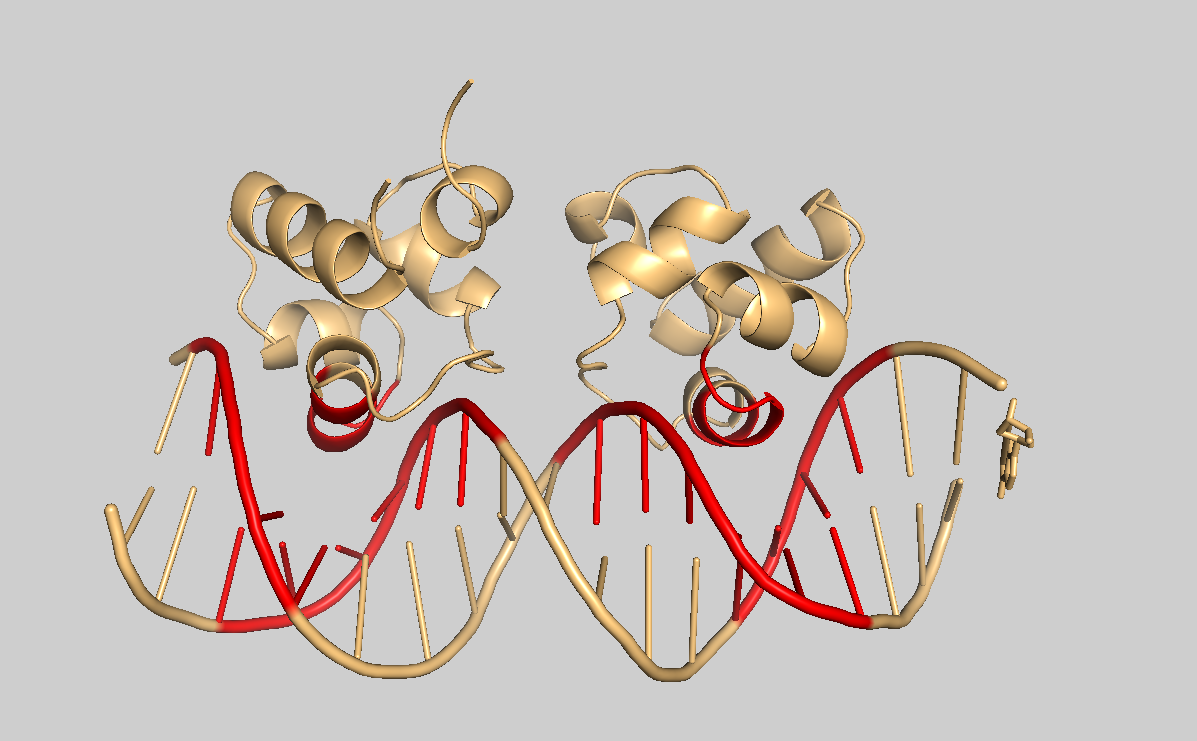
Let’s visualise residues in the interface of the 3CRO using PyMOL.
Open pdbs/3CRO_complex.pdb in PyMOL and type:
color lightorange, all
select interface, (chain A and resi 28+29+30+31+32+34+35, chain C and resi 28+29+30+31+32+34+35, chain B and resi 4+5+6+7+13+14+15+16+17+18+22+23+24+25+31+32+33+34+35+36)
color red, interface
Now the residues of the interface are displayed in red.expand_more
Let’s highlight the same residues on the unbound NRM structure of the protein.
Open PyMOL and type:
fetch 1ZUG
color lightorange, all
select region, (resi 28+29+30+31+32+34+35)
color red, region
set all_states, on
Answer expand_more
The conformation of the interacting region does not change in the ensemble, this region is not the most flexible. The most flexible region is the tail of the protein, and it appears to not interact with the DNA.
Let’s switch to the surface representation of a single model:
set all_states, off
show surface
Surface representation of a single model with interface residues highlighted in red.expand_more
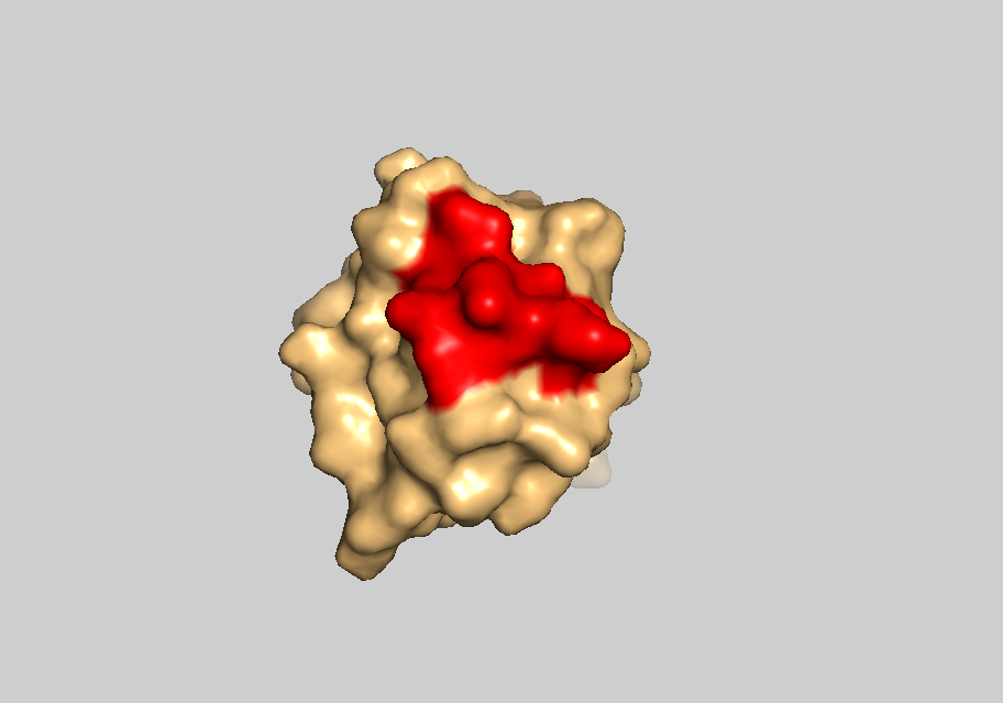
Can you tell why the residue 33 is excluded from the interface amino acids?
Answer expand_more
The residue 33 is not solvent accessible, thus it does not belong to the interface. You can visualise it by colouring residue 33 in blue, and switching between to the cartoon and surface representations (sele resi 33; color blue, sele; show cartoon; show surface)
Note that in the real docking case the bound structure of a complex is unavailable. In this case, the interface residues could be located using experimental data, knowledge from the literature, using computational predictions, etc.
What’s inside of the restraints file?
The ambiguous interaction restraints are defined in the ambig_prot_dna.tbl file.
This file was created using both experimental knowledge and information from literature.
A detailed explanation of how to generate these restraints can be found in the advanced version of the tutorial, accessible here.
Let’s have a look at it’s first lines:
assign ( resid 35 and segid C)
(
   (  resid 32 and segid B and (name H3 or name O4 or name C4 or name C5 or name C6 or name C7))
    or
    ( resid 33 and segid B and (name H3 or name O4 or name C4 or name C5 or name C6 or name C7))
) 2.000 2.000 0.000
The first line means that the residue 35 from the chain C (protein) should interact either with the residue 32, or with the residue 33 of the chain B (DNA). Additionally, the substring (name H3 or name O4 or name C4 or name C5 or name C6 or name C7) precise the atoms with which the interaction should occur.
To simplify, if at least one pair or residues (residue 35 from chain C; residue 32 from chain B) or (residue 35 from chain C; residue 33 from chain B) are located in the vicinity from one another - then this particular restraint is satisfied.
You may notice that not all residues of the protein’s interface are used for the AIRs. This is done to save computational time.
HADDOCK is not limited to ambiguous restraints, other types, like unambiguous and symmetry restraints can play an important role as well. As mentioned before, Cro is known to function as a symmetrical dimer. This means we should enforce a pairwise symmetry (C2) between the two protein monomers. This part will be explained in the Haddock3 workflow section of the tutorial.
Preparation of PDB files for the docking (optional)
Haddock3 requires an input structure for each docking partner. The quality of these input structures are highly influential to the quality of the docking models. Conformational deficiencies such as sterical clashes, chain breaks and missing atoms may cause problems during the docking, so it is important to verify each input file. Another important factor is the difference between unbound and bound conformations. The more different these conformations are, the more difficult it is to generate correct docking models.
In this section we will go over the preparation of the protein structures. The preparation of the DNA structure is out of the scope of this tutorial, but is detailed in the advanced tutorial.
Ready-to-dock structures are available in pdbs directory, namely 1ZUG_dimer1.pdb, 1ZUG_dimer2.pdb and OR1_unbound.pdb.
Protein structures
An unbound structure of the protein is available on PDB. We already examined this structure using PyMOL. Our observation revealed that this protein has a disordered tail, which does not interact with the DNA. Since the core conformation remains unchanged, we can simply take the first conformation from the ensemble, remove the disordered tail from it and use it as an input structure for the docking.
This can be done using pdb-tools, a collection of simple scripts handy to manipulate pdb files. pdb-tools is installed automatically with Haddock3. Alternatively, it is also available as a web-server.
To obtain a single trimmed structure, we will make use of the command-line version of pdb-tools.
Please, remember to activate a virtual environment for Haddock3 before using pdb-tools.
The following command will override the existing file with the name 1ZUG_dimer1.pdb - consider executing it outside of pdbs/:
pdb_fetch 1ZUG | pdb_selmodel -1 | pdb_delhetatm | pdb_selres -1:66 | pdb_tidy -strict > 1ZUG_dimer1.pdb
This sequence of commands: 1/ Downloads given structure in PDB format from the RCSB website; 2/ Extracts the first model from the file; 3/ Removes all HETATM records in the PDB file; 4/ Selects residues by their index (in a range); 5/ Adds TER statement at the end of the chain.
The complex of interest contains 2 copies of the protein. As each molecule given to HADDOCK in a docking scenario must have a unique chain ID and segment ID, we have to change the chain ID from A to C and save this as a new structure.
This can be achieved using another command from pdb_tools, namely, pdb_rplchain, which stands for “replace chain”:
pdb_rplchain -A:C 1ZUG_dimer1.pdb > 1ZUG_dimer2.pdb
Note that it is possible to perform the docking with an ensemble of trimmed conformations. Such ensemble can be obtained using the following command: pdb_fetch 1ZUG | pdb_delhetatm | pdb_selres -1:66 | pdb_tidy -strict > 1zug_ens.pdb. Here the command pdb_selmodel -1 was removed and therefore all the available models in the ensemble will be processed.
Docking with Haddock3
In this section, we will discuss the specificities related to protein-DNA docking in the frame of Haddock3. We will then create an appropriate Haddock3 workflow and, finally, perform an analysis of the docking results and evaluate their quality with respect to the experimentally solved structure as a reference.
Specifics of the protein-DNA docking
Docking a double-stranded DNA requires adjusting several default parameters to better mimic the conditions under which DNA interactions occur. The following parameters should be modified:
- Add an automatic restraint to maintain the input conformation of the DNA during refinement:
dnarest_on = true; - Perform explicit solvent molecular dynamics refinement instead of energy minimization refinement by using the
[mdref]module instead of[emref]; - Set the dielectric constant to 78 for both sampling and flexible refinement (but not for MD refinement):
epsilon = 78; - Fix the relative dielectric constant in the Coulomb potential (rather than using a distance-dependent mode) for both sampling and flexible refinement:
dielec = cdie; - Set the weight of the desolvation energy term to 0:
w_desolv = 0; - Lower the scaling factor for flexible refinement to 4 (from 8) to allow less movement during the refinement:
tadfactor = 4; - Lower the initial temperature for the final round of flexible refinement to 300 (from 1000) to allow less movement during the final refinement stage:
temp_cool3_init = 300.
Note that Haddock3 distinguishes DNA nucleotides from RNA nucleotides based on the residue naming in the PDB file. DNA nucleotides are named with two letters starting with ‘D’ (e.g., ‘DA’ for deoxyadenosine in DNA), while RNA nucleotides use single-letter names (e.g., ‘A’ for adenosine in RNA).
Haddock3 workflow
Now that we have all the necessary files ready for docking, along with several insights into the specifics of protein-DNA docking, it’s time to create the docking workflow. In this scenario, we will adhere to the following straightforward workflow: rigid-body docking, semi-flexible refinement in torsional angle space, molecular dynamics (MD) refinement in explicit solvent, and a final RMSD clustering step.
Our workflow consists of the following modules:
- topoaa: Generates the topologies for the CNS engine and builds missing atoms;
- rigidbody: Performs sampling by rigid-body energy minimization (equivalent to
it0in Haddock2.X); - caprieval: Calculates CAPRI metrics (i-RMSD, l-RMSD, Fnat, DockQ) with respect to the best-scored model or a provided reference structure;
- seletop: Selects X best-scored models from the previous module;
- flexref: Performs semi-flexible refinement of the interface (equivalent to
it1in Haddock2.X); - caprieval
- mdref: Performs final refinement via explicit solvent MD (equivalent to itw in Haddock2.X);
- caprieval
- rmsdmatrix: Calculates of the root mean squared deviation (RMSD) matrix between all models from the previous module;
- clustrmsd: Takes the RMSD matrix calculated in the
[rmsdmatrix]module and performs a hierarchical clustering procedure on it; - seletopclusts: Selects X best-scored models of Y clusters.
- caprieval: Final assessment of the docking results.
As mentioned before, we should enforce C2 symmetry between the proteins throughout the entire docking process. This can be easily achieved by adding the following parameters to the [rigidbody] , [flexref] , and [mdref] modules:
# Turn on symmetry restraints
sym_on = true
# Define first symmetry partner
c2sym_seg1_1 = 'A'
# Define second symmetry partner
c2sym_seg2_1 = 'C'
# Specify the range of residues that should be taken from the first partner
c2sym_sta1_1 = 4
c2sym_end1_1 = 64
# Specify the range of residues that should be taken from the second partner
c2sym_sta2_1 = 4
c2sym_end2_1 = 64
Note that in this definition we omitted the first 3 residues of each protein.
Take a look at the TOML configuration file protein-dna-basic.cfg.
# ====================================================================
# Protein-DNA basic docking example with:
# 1. Pre-generated ambiguous restraints between protein dimer and DNA partners
# 2. Pairwise (C2) symmetry between the two protein monomers
# 3. Specific to double-stranded DNA-protein docking parameters
# ====================================================================

# directory in which the docking will be performed
run_dir = "run"

# compute mode
mode = "local"
ncores = 8

# input PDBs of the docking partners
molecules =  [
    "pdbs/1ZUG_dimer1.pdb",
    "pdbs/OR1_unbound.pdb",
    "pdbs/1ZUG_dimer2.pdb"
    ]

# compress all generated models
clean = true

# ====================================================================
# Workflow is defined as a pipeline of modules with specified parameters per module
# ====================================================================

[topoaa]

[rigidbody]
# allow up to 5% of the models to fail without interrupting the run
tolerance = 5
# create 1000 modles (default value)
sampling = 1000
# Cro to OR1 ambiguous restraints
ambig_fname = "restraints/ambig_prot_DNA.tbl"
# C2 symmetry
sym_on = true
c2sym_seg1_1 = 'A'
c2sym_seg2_1 = 'C'
c2sym_sta1_1 = 4
c2sym_sta2_1 = 4
c2sym_end1_1 = 64
c2sym_end2_1 = 64
# constant for the electrostatic energy term
epsilon = 78
# fix constant in Coulomb potential
dielec = 'cdie'
# weight of the desolvation energy term
w_desolv = 0

[caprieval]
reference_fname = "pdbs/3CRO_complex.pdb"

[seletop]
# select top 200 models (default value) based on HADDOCK score
select = 200

[flexref]
tolerance = 5
# to maintain conformation of the DNA with automatic restraints
dnarest_on = true
# Cro to OR1 ambiguous restraints
ambig_fname = "restraints/ambig_prot_DNA.tbl"
# C2 symmetry
sym_on = true
c2sym_seg1_1 = 'A'
c2sym_seg2_1 = 'C'
c2sym_sta1_1 = 4
c2sym_sta2_1 = 4
c2sym_end1_1 = 64
c2sym_end2_1 = 64
# constant for the electrostatic energy term
epsilon = 78
# fix constant in Coulomb potential
dielec = 'cdie'
# weight of the desolvation energy term
w_desolv = 0
# allow less movement during the refinement
tadfactor = 4
# reduce the initial temperature for the final round of flexible refinement to 300 (from 1000 with default parameters)
temp_cool3_init = 300

[caprieval]
reference_fname = "pdbs/3CRO_complex.pdb"

[mdref]
tolerance = 5
# to maintain conformation of the DNA with automatic restraints
dnarest_on = true
# Cro to OR1 ambiguous restraints
ambig_fname = "restraints/ambig_prot_DNA.tbl"
# C2 symmetry
sym_on = true
c2sym_seg1_1 = 'A'
c2sym_seg2_1 = 'C'
c2sym_sta1_1 = 4
c2sym_sta2_1 = 4
c2sym_end1_1 = 64
c2sym_end2_1 = 64
# constant for the electrostatic energy term (default value)
epsilon = 1
w_desolv = 0
# reduce the number of MD steps
watersteps = 750

[caprieval]
reference_fname = "pdbs/3CRO_complex.pdb"

[rmsdmatrix]
# by default, all residues of each docking partner are used to calculate the RMSD matrix

[clustrmsd]
# generate an interactive plot of the clustering results
plot_matrix = true
# reduce the clustering cutoff distance from 7.5
clust_cutoff = 5.5

[seletopclusts]

[caprieval]
reference_fname = "pdbs/3CRO_complex.pdb"

# ====================================================================
Note that in this example we use relative paths to define input files and output folder. However it is preferable to use the full paths instead.
This workflow begins by creating topologies for the docking partners ([topoaa]). Rigid body sampling ([rigidbody]) is performed with ambiguous and symmetry restraints, generating 1000 models, from which the top 200 are selected ([seletop]). These models then undergo flexible refinement ([flexref]) followed by MD refinement in explicit solvent ([mdref]), still maintaining the same ambiguous and symmetry restraints. Finally, the RMSD matrix for docking models is computed ([rmsdmatrix]), followed by its clusterisation ([clustrmsd]). The RMSD values are calculated using the backbone atoms of all residues of each docking partner. The top 10 models from each cluster are selected ([seletopclusts]). The caprieval module is added after each step using the crystal structure as a reference to simplify the analysis and track the rank of models throughout the docking process.
Running Haddock3 locally
In the first section of the configuration file you can see the definition of the global parameters:
# compute mode
mode = "local"
ncores = 8
The parameter mode defines how this workflow will be executed. In this case, it will run locally, on your machine, using up to 8 CPUs. Feel free to change this value, if more cores are available. You can find out about other modes here.
To start the docking you need to activate your haddock3 environment, then navigate to the folder haddock3-protein-dna-basic with the configuration file protein-dna-basic.cfg, and type one of the following:
haddock3 protein-dna-basic.cfg > log-protein-dna-basic.out &
or
haddock3 protein-dna-basic.cfg
The first version of this command will run the docking in the background and will save output in the file log-protein-dna-basic.out, i.e. you will be able to close the terminal window without terminating the docking. The second version will run directly in the terminal window and will print output on the screen, so you will have to leave the terminal window open while Haddock3 is running.
This workflow took 1.5 hours to complete using 8 CPUs (on an Apple M3 laptop). You can run it and wait for the results, or you can access pre-computed results of this protocol immediately by navigating to the precomputed directory.
Analysis of the docking results
Let’s get acquainted with the contents of the resulting directory - take a look inside. You will find that the various steps of our workflow (modules) are numbered sequentially, starting at 0:
> ls precomputed/
     00_topoaa/
     01_rigidbody/
     02_caprieval/
     03_seletop/
     04_flexref/
     05_caprieval/
     06_mdref/
     07_caprieval/
     08_rmsdmatrix/
     09_clustrmsd/
     10_seletopclusts/
     11_caprieval/
     analysis/
     data/
     log
     traceback/
Additionally, you will find the following directories and files:
logfile: This file allows you to verify the execution of each module. More importantly, if the docking run fails, you can identify the cause by carefully reading the error messages. Also, at the very bottom of the file, you can see the total execution time of the docking run;analysisdirectory: Contains information relevant to the results of each caprieval step, including filereport.htmlwith thee table containing limited number of the top-ranked models/clusters and various plots to visualise statistics of the results;datadirectory: Stores input PDB files (not the actual docking models) and restraints files used in each module;tracebackdirectory: Contains thetraceback.tsvfile, which tracks the name and rank of each docking model throughout the entire workflow. Handy, if you want to see how the model’s rank evolved step-by-step.
Each sampling, refinement, or selection module’s directory contains compressed PDB files of the docking models. For example, 10_seletopclusts contains 10 top-ranked docking models from each of the 4 clusters. Clusters are numbered based on the average rank of the models within them, so cluster_1 contains the top-ranked models of the entire run. Information about the origin of each model can be found in 10_seletopclusts/seletopclusts.txt, as well as in traceback/traceback.tsv.
One of the ways to analyse the docking results is to examine file(s) analysis/XX_caprieval_analysis/report.html. Depending on the positionning of the given caprieval module, report.html will display information about the models at the different stages of the workflow. For example, 11_caprieval_analysis/report.html contains statictis related of the clusters, while 02_caprieval_analysis/report.html contains statictis related to the models generated during the rigid body sampling stage.
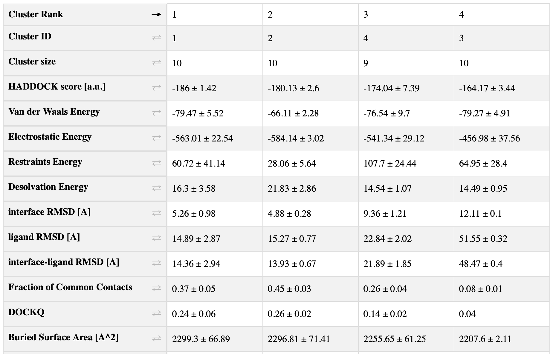
Caprieval, executed after clustering - in this case 11_caprieval - enables a comprehensive evaluation of the docking results from a broad perspective.
Here is a screenshot of the top-left corner of the table in 11_caprieval_analysis/report.html:
You can also access this file here.
Answer expand_more
According to the two-sample t-test, there is a significant difference between all 3 clusters.
In this docking case, we had access to the experimentally solved structure of the complex, which we provided to all [caprieval] modules using the reference_fname parameter. As a result, the interface RMSD (i-RMSD), ligand RMSD (l-RMSD), Fraction of Common Contacts (FCC), and DockQ statistics reflect the quality of the docked model with respect to the reference structure.
Remember that high DockQ and FCC values, along with low RMSD values, indicate better model quality.
Look at the DockQ of the clusters: Does the top-ranked cluster have the highest average DockQ?
Answer expand_more
No, cluster_2 has the highest average DockQ equal to 0.26+/-0.02.
Note that if no reference structure is provided to the caprieval module, all statistics are calculated relative to the top-ranked (based on HADDOCK score) docking model. However, keep in mind that the top-ranked model may not necessarily represent the true solution.
Visualisation of the HADDOCK scores and their components
Below the cluster statistics table, you’ll find a series of plots displaying the HADDOCK score and its components against various metrics (i-RMSD, l-RMSD, FCC, DockQ), with clusters represented using color coding. The last rows show plots of cluster statistics, i.e. distributions of values per cluster, ordered by their HADDOCK score.
These plots are interactive. A menu will appear at the top right, just above the last plot in the first row, when you hover your mouse over it. This menu allows you to zoom in and out of the plots and toggle the visibility of clusters.
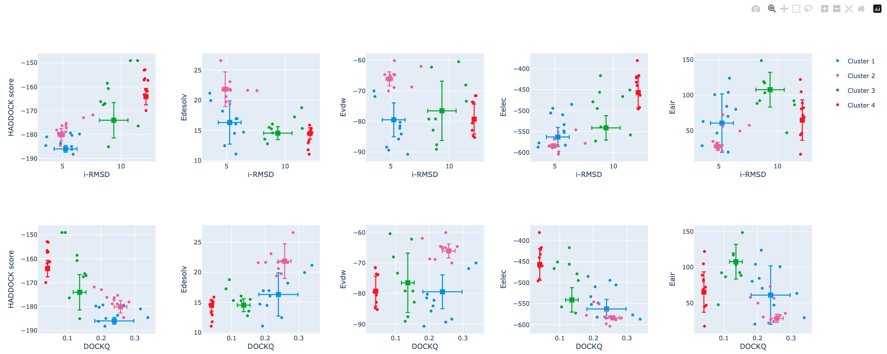
Inspect the plots. Which of the score components correlates best with the quality of the models?
Depending on the docking models, there could be a set of unclustered models. It will be explicitly shown in report.html as ‘other’. You can see the origins of these models in traceback/traceback.tsv.
Visualisation of the docking models
It’s time to visualise some of the docking models. Let’s take a look at cluster_1_model_1.pdb.gz, the best-ranked model; cluster_1_model_4.pdb.gz, the model with the lowest i-RMSD (as shown in the plot “HADDOCK score vs i-RMSD”); and the reference structure 3CRO_complex.pdb. Please open all these files in PyMOL (it can display compressed PDB files). You can find the first two files in 10_seletopclusts, and the reference structure in pdbs. Then, in the PyMOL command line, type:
show cartoon color paleyellow, 3CRO_complex align cluster_1_model_1 and chain B, 3CRO_complex and chain B align cluster_1_mode_4 and chain B, 3CRO_complex and chain B
See the overlay of the top ranked model onto the reference structure.expand_more
Reference structure is displyed in yellow; cluster_1_model_1 in green; cluster_1_model_4 in blue.
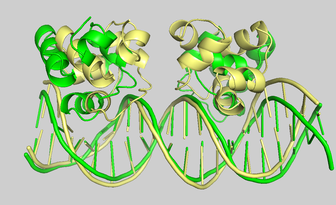
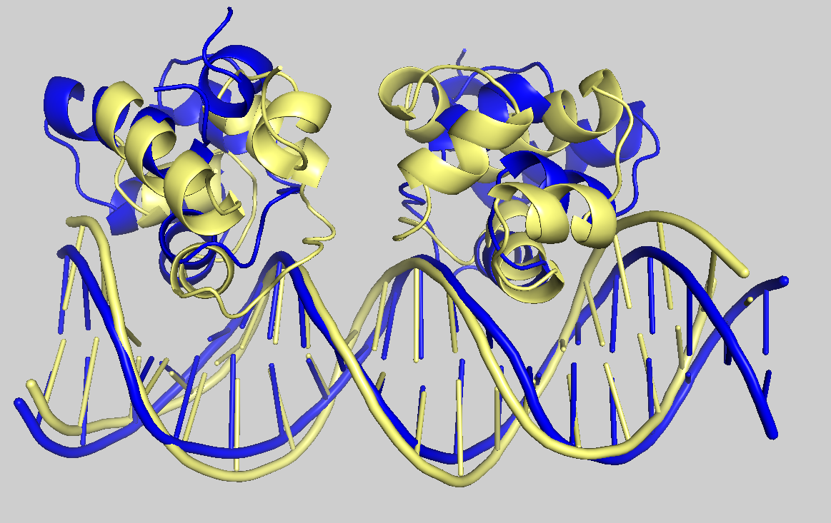
Note that models are compressed because of the line clean = true in the global parameters of the workflow. To decompress all models in a directory, one can run haddock3-unpack <path/to/directory>
Answer expand_more
The models are acceptably close to the reference. Although the best model may not be top-ranked one, HADDOCK produces a reasonable ranking.
It may be helpful to examine several top-ranked models from each cluster. This can give you insight into the diversity of the models within a cluster, as well as the diversity of models across different clusters.
Congratulations!
You’ve reached the end of this basic protein-DNA docking tutorial. We hope it has been informative and helps you get started with your own docking projects. Check out the advanced version of this tutorial (currently awaliable only for Haddock2.4 server) for deeper insights into protein-DNA docking!
Happy docking!

