

Protein-glycan modelling tutorial using a local version of HADDOCK3
This tutorial consists of the following sections:
- Introduction
- Requirements
- Preparing PDB files for docking
- Defining restraints for docking
- Setting up the docking with HADDOCK3
- Analysis of docking results
- Visualisation and comparison with the reference structure
- Conclusions
- BONUS1: Using an ensemble of glycan conformations
- BONUS2: Modifying the scoring weights at the flexible refinement stage
Introduction
This tutorial demonstrates the use of HADDOCK3 for predicting the structure of a protein-glycan complex using information about the protein binding site.
A glycan is a molecule composed of different monosaccharide units, linked to each other by glycosidic bonds. Glycans are involved in a wide range of biological processes, such as cell-cell recognition, cell adhesion, and immune response. Glycan are highly diverse and complex in their structure, as they can involve multiple branches and different linkages, namely different ways in which a glycosidic bond can connect two monosaccharides. This complexity together with their flexibility makes the prediction of glycan-protein interactions a challenging task.
In this tutorial we will be working with the catalytic domain of the Humicola Grisea Cel12A enzyme (PDB code 1OLR) and a linear homopolymer, 4-beta-glucopyranose, as glycan (PDB code of the complex 1UU6).
The tutorial is based on A. Ranaudo et al., J. Chem. Inf. Model. 64 (19), 7816-7825, 2024.
Throughout the tutorial, colored text will be used to refer to questions or instructions, and/or PyMOL commands.
This is a question prompt: try answering it! This an instruction prompt: follow it! This is a PyMOL prompt: write this in the PyMOL command line prompt! This is a Linux prompt: insert the commands in the terminal!
Requirements
In order to follow this tutorial you will need to work in a Linux terminal. We will also make use of PyMOL (freely available for most operating systems) in order to visualize the input and output data. We will provide you links to download the various required software and data. We assume that you have a working installation of HADDOCK3 on your system.
In case HADDOCK3 is not pre-installed in your system you will have to install it. To obtain HADDOCK3, fill the registration form, and then follow the installation instructions.
Further we are providing pre-processed PDB files for docking and analysis (but the preprocessing of those files will also be explained in this tutorial). The files have been processed to facilitate their use in HADDOCK and for allowing comparison with the known reference structure of the complex. For this download and unzip the following zip archive and note the location of the extracted PDB files in your system. Once unzipped, you should find the following directories:
haddock3: Contains HADDOCK3 configuration and job files for the various scenarios in this tutorialpdbs: Contains the pre-processed PDB filesplots: Contains pre-generated html plots for the various scenarios in this tutorialrestraints: Contains the interface information and the corresponding restraint files for HADDOCKruns: Contains pre-calculated run results for the various scenarios in this tutorial
Preparing PDB files for docking
In this section we will prepare the PDB files of the protein and glycan for docking. A crystal structure of the protein in the unbound form is available, but you are welcome to use either the bound form or the Alphafold structure if you prefer.
Note: Before starting to work on the tutorial, make sure to activate haddock3. For example, if haddock3 was installed using conda
Preparing the protein structure
Using PDB-tools we will download the structure from the PDB database (the PDB ID is 1OLR) and then process it to remove water and heteroatoms.
This can be done from the command line with:
The command fetches the PDB ID and removes water and heteroatoms (in this case no co-factor is present that should be kept).
Note that the corresponding files can be found in the pdbs directory of the archive you downloaded.
Preparing the glycan structure
We will model the glycan using the GLYCAM webserver. Our glycan is a linear polymer consisting of 4 beta-D-glucopyranose units. Beta-D-glucopyranose is a common monosaccharide found basically in all the living organisms. In this case the four monosaccharides are linked by beta-1,4-glycosidic bonds, where the anomeric carbon (C1) of one monosaccharide is linked to the C4 of the next one.
We can start by accessing the GLYCAM webserver where we will model the glycan!
Select the Glc monosaccharide with your mouse.
This will add the monosaccharide to the sequence, together with an OH group as aglycon (the non-sugar part of a glycan).
Now we need to add a second beta-D-glucopyranose unit to the sequence. We will link it to the first one by a beta-1,4-glycosidic bond.
Click one more time on the Glc icon.
Now you are asked to specify a linkage.
Select the Beta linkage and the 1-4 option. Do not change the other parameters.
This will add the second monosaccharide to the sequence, linked to the first one by a beta-1,4-glycosidic bond.
Repeat the process to add the third and fourth monosaccharide units to the sequence.
At the end of the process you should observe the following sequence:
DGlcpb1-4DGlcpb1-4DGlcpb1-4DGlcpa1-OH
Unfortunately, the glycan structure we just obtained cannot be directly used in HADDOCK as the formant and the residue and atom naming differ from the conventions used in HADDOCK (which follow the naming in the PDB). We will need to edit it to remove the several TER statements GLYCAM placed between the monosaccharides, and to add the HADDOCK residue name proper to beta-D-glucopyranose. Importantly, we have to merge the OH aglycon with the first monosaccharide unit, as they are now separated in two different residues.
What is the HADDOCK three letter code corresponding to beta-D-glucopyranose?
Let us start with the aglycon:
This command selects the GLYCAM residue name proper to the aglycon, changes the chain ID to B, and changes the residue name to the HADDOCK one. The final structure is saved in the aglycon.pdb file. Now we will process the rest of the glycan structure:
The pdb_tidy command removes the TER statements between each unit, while pdb_selres selects all the residues except the OH aglycon. The pdb_chain command changes the chain ID to B, and the pdb_rplresname command changes the residue name to BGC. The last command, pdb_reres, renumbers the residues of the glycan starting from 1.
We will now merge the two structures in the 1UU6_l_u.pdb file:
pdb_merge aglycon.pdb sugar.pdb | pdb_tidy > 1UU6_l_u.pdb
Note that the pre-processed glycan structure can be found in the pdbs directory of the archive you downloaded.
Now we would like to know how close the modelled glycan is to the reference structure. For this we will use Pymol to superimpose the two structures and calculate the RMSD. Start pymol and then load the generated PDB file from the file menu (alternatively start it from the command line with as argument the name of the PDB file):
File menu -> Open -> select 1UU6_l_u.pdb
Defining restraints for docking
Visualising the information about the binding site
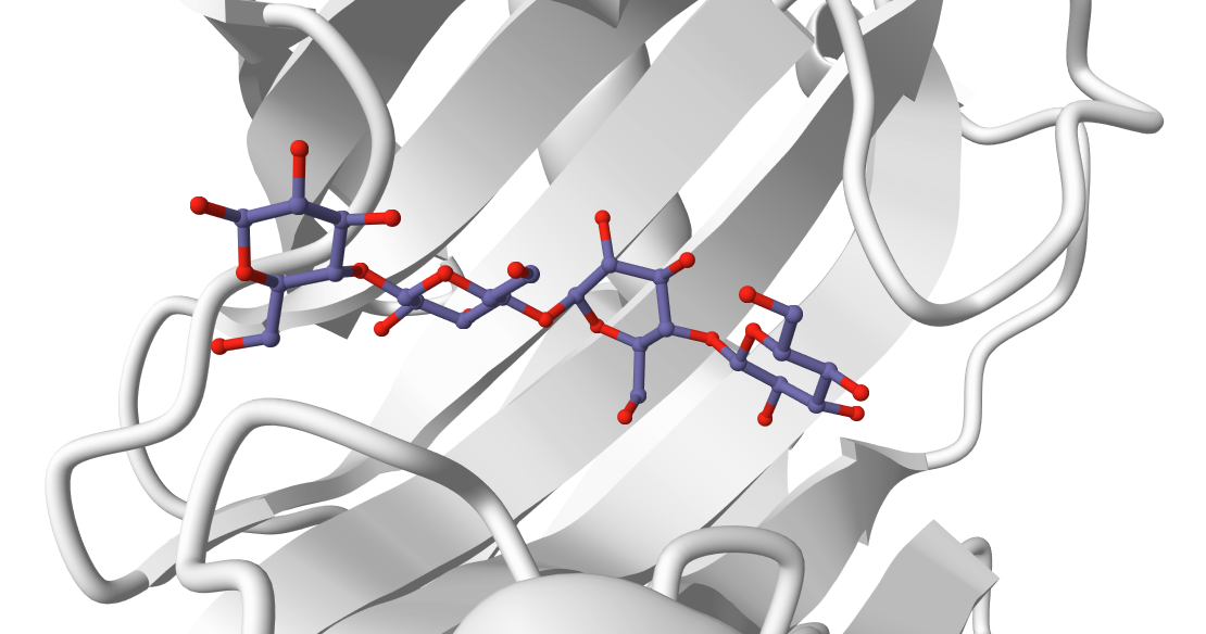
Here we mimic a scenario where we have information about the glycan binding site on the protein, but no knowledge about which monosaccharide units are relevant for the binding. In this case (see Fig. 1), all the four beta-D-glucopyranose units are at the interface, although this might not be true in general, especially when longer glycans are considered.
The following residues correspond to the protein binding site, as calculated from the crystal structure of the complex are:
22,24,59,64,97,103,105,115,120,122,124,131,132,133,134,155,158,205,207
Let us visualize the interface on our unbound protein structure. For this start PyMol and load the PDB file of the unbound protein:
File menu -> Open -> select 1OLR_clean.pdb
color white, all
select binding_site, (resi 22+24+59+64+97+103+105+115+120+122+124+131+132+133+134+155+158+205+207)
color red, binding_site
In order to visualize the binding site of a small molecule we have to add the side chains to our representation.
Are all the highlighted side chains exposed on the surface of the protein?
Note that you can visualise the surface in PyMol with the following command:
Generating the restraints
In this section we will define the restraints that will guide the docking of the protein and glycan structures.
A description of the format for the various restraint types supported by HADDOCK can be found in our Nature Protocol paper, Box 1. Information about various types of distance restraints in HADDOCK can also be found in our online manual pages.
We will use haddock3-restraints to generate the restraints for the protein-glycan docking.
For this we need to define two files, one for each molecule, containing on the first line the list of active residues
(those that should be at the interface) and on the second line the list of passive residues (those that can be at the interface).
For the protein, we will only define active residues (based on the identified binding site above) and leave the second line (passive) empty, while for the glycan we only define passive residues in the second line, leaving the first line empty. The corresponding files are provided as:
- restraints/1olr-binding-site.act for the protein
- restraints/glycan.pass for the glycan
The command to generate a HADDOCK ambiguous distance restraint file (.tbl) from those file is:
We can check the validity of the generated tbl file (useful when manually editing restraint files) with:
haddock3-restraints validate_tbl ambig.tbl
No output means that your TBL file is valid.
Inspect the generated file. Can you understand the syntax?
What is the distance range (lower and upper limits) defined for the restraints?
Distance restraints in the HADDOCK/CNS syntax are defined as:
assign (selection1) (selection2) distance, lower-bound correction, upper-bound correction
where the lower limit for the distance is calculated as: distance minus lower-bound correction
and the upper limit as: distance plus upper-bound correction.
Setting up the docking with HADDOCK3
Now that we have all required files at hand (PDB and restraints files) it is time to setup our docking protocol. For this we need to create a HADDOCK3 configuration file that will define the docking workflow. We will illustrate this flexibility by introducing a clustering step after the initial rigid-body docking stage, select up to 20 models per cluster and refine all of those.
HADDOCK3 also provides an analysis module (caprieval) that allows
to compare models to either the best scoring model (if no reference is given) or to a reference structure, which in our case
we have at hand.
The basic workflow for all three scenarios will consists of the following modules, with some differences in the restraints used and some parameter settings (see below):
topoaa: Generates the topologies for the CNS engine and build missing atomsrigidbody: Rigid body energy minimisation (it0in haddock2.x)caprieval: Calculates CAPRI metrics (i-RMSD, l-RMSD, Fnat, DockQ) with respect to the top scoring model or reference structure if providedilrmsdmatrix: Calculate the ilRMSD matrix between the generated modelsclustrmsd: Cluster the ilRMSD matrix in 50 clustersseletopclusts: Selection of the top20 models of each clusterscaprieval: Calculates CAPRI metrics (i-RMSD, l-RMSD, Fnat, DockQ) with respect to the top scoring model or reference structure if providedflexref: Semi-flexible refinement of the interface (it1in haddock2.4)caprieval: Calculates CAPRI metrics (i-RMSD, l-RMSD, Fnat, DockQ) with respect to the top scoring model or reference structure if providedilrmsdmatrix: Calculate the ilRMSD matrix between the generated modelsclustrmsd: Cluster the ilRMSD matrixseletopclusts: Selection of the top4 models of all clusterscaprieval: Calculates CAPRI metrics (i-RMSD, l-RMSD, Fnat, DockQ) with respect to the top scoring model or reference structure if provided
The configuration file for this scenario is already provided in the haddock3 directory of the archive you downloaded, together with different examples related to the different execution modes of HADDOCK3 (for a comprehensive description see the antibody-antigen tutorial).
# ====================================================================
# protein-glycan docking using information about the protein binding site
# and no information on the glycan side
# ====================================================================
#general section
mode = "local"
ncores = 10
run_dir = "run_prot-glyc"  #insert full path

# list, insert full path
molecules = [
    "../pdbs/1OLR_clean.pdb",
    "../pdbs/1UU6_l_u.pdb",
]

[topoaa]

[rigidbody]
ambig_fname = "../restraints/ambig.tbl"
w_vdw = 1

[caprieval]
reference_fname = "../pdbs/1UU6_target.pdb"

[ilrmsdmatrix]

[clustrmsd]
criterion = 'maxclust'
n_clusters = 50

[seletopclusts]
top_models = 20

[caprieval]
reference_fname = "../pdbs/1UU6_target.pdb"

[flexref]
ambig_fname = "../restraints/ambig.tbl"
tolerance = 5

[caprieval]
reference_fname = "../pdbs/1UU6_target.pdb"

[ilrmsdmatrix]

[clustrmsd]
criterion = 'distance'
linkage = 'average'
min_population = 4
clust_cutoff = 2.5

[seletopclusts]
top_models = 4

[caprieval]
reference_fname = "../pdbs/1UU6_target.pdb"
Important : the weight of the van der Waals component of the HADDOCK score at the rigidbody stage has been set to 1.0
rather than the default 0.01 (vdw_w = 1.0) as in the protein-protein tutorial. This is in agreement with the settings
used for protein-small molecules docking in HADDOCK2.4, as explained in Journal of Computer-Aided Molecular Design, 2019 and also applied to protein-glycan docking.
Note that the clustering step is placed between the rigidbody and the flexible refinement stages.
This was not possible in the static workflow proper to the HADDOCK2.X series, but is now doable in HADDOCK3.
The idea here is that the scoring function at the rigidbody level is not perfect, thus good models may not be selected
if we only consider the top 200 models (as in HADDOCK2.X). Clustering the rigidbody models
(1000 generated with default settings - can be changed by adding a sampling parameter in the rigid body module)
allows to increase the diversity of the models selected for the flexible refinement stage.
If you have everything ready, you can launch haddock3 either from the command line, or, better, submitting it to
the batch system requesting in this local run mode a full node and adapting the ncores parameter to the number of cores avaible on a node.
Make sure to launch this command from the haddock3 directory in the data directory downloaded for this tutorial.
If you do not wish to wait for the run to finish, you can find the (partial) results of the run in the runs/run_prot-glyc directory of the archive you downloaded.
Analysis of docking results
Inspecting the results of the docking run
Once your run has completed inspect the content of the resulting directory. You will find the various steps (modules) of the defined workflow numbered sequentially, e.g.:
> ls run_prot-glyc/
  00_topoaa
  01_rigidbody
  02_caprieval
  03_ilrmsdmatrix
  04_clustrmsd
  05_seletopclusts
  06_caprieval
  07_flexref
  08_caprieval
  09_ilrmsdmatrix
  10_clustrmsd
  11_seletopclusts
  12_caprieval
  analysis
  data
  log
  traceback
There is in addition to the various modules defined in the config workflow a log file (text file) and three additional directories:
- the
datadirectory containing the input data (PDB and restraint files) for the various modules - the
analysisdirectory containing various plots to visualise the results for eachcaprievalstep - the
tracebackdirectory containing the names of the generated models for each step, allowing to trace back a model throughout the various stages.
You can find information about the duration of the run at the bottom of the log file. Each sampling/refinement/selection module will contain PDB files.
For example, the 11_seletopclusts directory contains the selected models from each cluster. The clusters in that directory are numbered based
on their rank, i.e. cluster_1 refers to the top-ranked cluster. Information about the origin of these files can be found in that directory in the seletopclusts.txt file.
The simplest way to extract ranking information and the corresponding HADDOCK scores is to look at the X_caprieval directories (which is why it is a good idea to have it as the final module, and possibly as intermediate steps, even when no reference structures are known). This directory will always contain a capri_ss.tsv file, which contains the model names, rankings and statistics (score, iRMSD, Fnat, lRMSD, ilRMSD and dockq score). E.g.:
model                         md5 caprieval_rank  score         irmsd    fnat   lrmsd   ilrmsd  dockq      cluster_id      cluster_ranking model-cluster_ranking   air     angles     bonds   bsa     cdih    coup    dani    desolv  dihe    elec    improper   rdcs    rg      sym     total   vdw     vean    xpcs
../07_flexref/flexref_139.pdb   -       1       -171.128        4.483   0.318   12.677  12.670  0.243   -       -       -       34.993  0.000   0.000   914.696 0.000      0.000   0.000   -1.980  0.000   -132.565        0.000   0.000   0.000   0.000   -128.507        -30.936 0.000   0.000
../07_flexref/flexref_222.pdb   -       2       -168.406        1.450   0.614   4.089   4.087   0.648   -       -       -       34.083  0.000   0.000   951.757 0.000      0.000   0.000   -6.838  0.000   -115.378        0.000   0.000   0.000   0.000   -121.376        -40.081 0.000   0.000
../07_flexref/flexref_216.pdb   -       3       -164.403        4.183   0.273   11.677  11.675  0.244   -       -       -       0.886   0.000   0.000   1024.660  0.000    0.000   0.000   -3.221  0.000   -104.942        0.000   0.000   0.000   0.000   -150.138        -46.082 0.000   0.000
../07_flexref/flexref_71.pdb    -       4       -158.462        0.942   0.727   2.482   2.486   0.789   -       -       -       25.864  0.000   0.000   1056.530  0.000    0.000   0.000   -8.386  0.000   -94.870 0.000   0.000   0.000   0.000   -116.233        -47.227 0.000   0.000
../07_flexref/flexref_142.pdb   -       5       -158.083        4.418   0.318   12.484  12.477  0.246
....
The iRMSD, lRMSD and Fnat metrics are the ones used in the blind protein-protein prediction experiment CAPRI (Critical PRediction of Interactions).
In CAPRI the quality of a model is defined as (for protein-protein complexes):
- acceptable model: i-RMSD < 4Å or l-RMSD<10Å and Fnat > 0.1
- medium quality model: i-RMSD < 2Å or l-RMSD<5Å and Fnat > 0.3
- high quality model: i-RMSD < 1Å or l-RMSD<1Å and Fnat > 0.5
As these metrics are for protein-protein complexes and glycans are typically smaller, it is best to use stricter metrics to assess the quality of the models. In the case of information-driven protein-glycan docking, the Fnat term is less relevant, as most contacts will typically be satisfied.
For protein-glycan modelling we recently proposed a different, stricter metric based on the interface ligand RMSD (ilRMSD), see A. Ranaudo et al., J. Chem. Inf. Model. 64 (19), 7816-7825, 2024:
- near acceptable model: ilRMSD < 4Å
- acceptable model: ilRMSD < 3Å
- medium quality model: ilRMSD < 2Å
- high quality model: ilRMSD < 1Å
The ilRMSD is calculated by fitting the models onto the refence using the interface residues of the receptor (the protein in this case) and calculated the RMSD on the ligand (the glycans in this case).
What is based on this criterion the quality of the top ranked model listed above (flexref_139.pdb)? Consider now the model with the best ilRMSD (lowest value). Which model is it and what is its quality?
Near-acceptable quality models can be considered OK for long linear glycans (like the one we are using here), but for smaller glycans the quality of the models should be higher.
Since we have caprieval steps at various stages of the workflow we can assess the impact of the flexible refinement.
The ilRMSD values are listed in column 8 of the capri_ss.tsv file. To find the lowest ilRMSD value you can sort the file numerically based on column 8 and extract the top model.
This can be down at the command line with the following command:
sort -nk8 capri_ss.tsv | head -2
Visualising the scores and their components
The HADDOCK3 analysis precalculated a lot of plots and tables for you to inspect the results.
You can find them in the analysis directory of each run, with one folder available for each caprieval step.
The plots are in html format and can be opened in your browser. You can also open the full report in your browser:
python -m http.server --directory ./run_prot-glyc
and then open your browser at http://localhost:8000/analysis/. From there you can navigate to the preferred caprieval directory (typically the last one), to inspect the results.
Under a given caprieval step, the overall view of the results can be found in the report.html file.
If this does not work (for example because port 8000 is already in use), you can also open the html files directly from the file system. For example, to inspect the final results (after refinement):
open run_prot-glyc/analysis/12_caprieval_analysis/report.html
Alternatively, you can check this example report for the final docking results.
Visualisation and comparison with the reference structure
To visualize the models from top cluster of your favorite run, start PyMOL and load the cluster representatives you want to view,
e.g. this could be the top model from cluster1. These can be found in the runs/run_prot-glyc/11_seletopclusts/ directory.
Let us unzip the files: gunzip -d run_prot-glyc/11_seletopclusts/cluster_*.pdb.gz
You can load the models from the run_prot-glyc/11_seletopclusts directory in PyMOL.
Will first check the top ranked cluster to see if this is good solution.
File menu -> Open -> cluster_1_model_1.pdb
If you want to get an impression of how well defined a cluster is, repeat this for the best N models you want to view (cluster_1_model_X.pdb).
From the pdbs directory we can load the reference structure: File menu -> Open -> 1UU6_target.pdb
Once all files have been loaded, type in the PyMOL command window:
show cartoon
util.cbc
color yellow, 1UU6_target
util.cnc
Let us then superimpose all models on the reference structure:
This will align the proteins. To evaluate the quality of the glycan pose, we can now calculate the ligand-RMSD (l-RMSD) between the glycan in the model and the reference structure. This can be done with the following, superimposition-free PyMOL command:
rms_cur 1UU6_target and chain B,cluster_1_model_1 and chain B
Did the glycan conformation improve thanks to the refinement in any of the selected models?
To address this question you can use the standard align command, focusing on chain B:
align cluster_1_model_1 and chain B, 1UU6_target and chain B, cycles=0
Now repeat this analysis but with the cluster with the lowest ilRMSD values.
How close are the top4 models of this cluster to the reference? What was the rank of this cluster?
Let’s now check if the active residues which we have defined (the protein binding site) are actually part of the interface. In the PyMOL command window type:
Are the residues of the binding_site at the interface with the glycan?
Note: You can turn on and off a model by clicking on its name in the right panel of the PyMOL window.
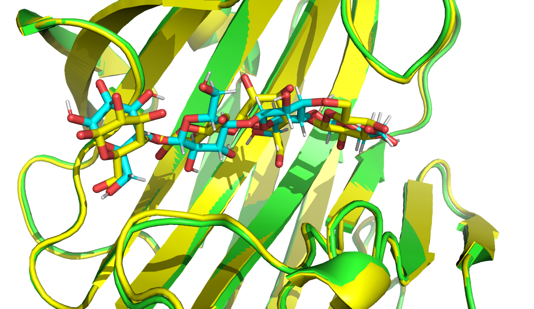
See the overlay of the cluster solution with the lowest ilRMSD values (ranked #2) onto the reference crystal structure (in yellow)
Conclusions
In this tutorial we have demonstrated the use of HADDOCK3 to predict the structure of a protein-glycan complex using information about the protein binding site. We have shown how to prepare the PDB files for docking, define the restraints, and set up the docking protocol. We have also discussed the analysis of the docking results and the comparison with the reference structure.
We hope you have enjoyed this tutorial and that you have learned something new. If you have any questions or feedback, please do not hesitate to contact us on the HADDOCK forum.
BONUS1: Using an ensemble of glycan conformations
Creating an ensemble of glycan conformations
We have just modelled a single conformation of the glycan. However, glycans are highly flexible molecules that can adopt multiple conformations. Indeed, the modelled glycan is quite different from the conformation adopted in the reference structure. To account for this flexibility, we can generate an ensemble of glycan structures that will be docked to the protein.
To do this, we will use the short Molecular Dynamics refinement protocol available in HADDOCK3. This protocol will generate an ensemble of glycan conformations by running short MD simulations on the glycan structure. The hope here is to observe a glycan structure that is significantly closer to the structure observed in the complex (bound conformation). You are encouraged to try more extensive and optimized MD software for this task, such as GROMACS and OPENMM, but for the sake of this tutorial, we will use HADDOCK3.
We will use the following protocol, available as glycan-mdref.cfg in the haddock3 directory of the archive you downloaded:
# ====================================================================
# MD Refinment of the glycan conformation
# ====================================================================
run_dir = "run-glycan-mdref"

# execution mode
mode = "local"
ncores = 10

# starting glycan conformation
molecules =  [
    "../pdbs/1UU6_l_u.pdb",
    ]

# ====================================================================
# Parameters for each stage are defined below, prefer full paths
# ====================================================================
[topoaa]

[mdref]
tolerance = 5
nfle1 = 1
fle_sta_1_1 = 1
fle_end_1_1 = 4
sampling_factor = 20
nemsteps = 200
waterheatsteps = 100
watersteps = 20000
watercoolsteps = 8000

[rmsdmatrix]

[clustrmsd]
criterion = 'distance'
linkage = 'average'
min_population = 1
clust_cutoff = 0.6

[seletopclusts]
top_models = 1
This protocol will run a short MD simulation on the glycan structure, generate an ensemble of conformations, cluster them based on their RMSD using a 0.6Å cutoff, and select the cluster center from each cluster.
Note how the glycan is here defined as fully flexible (nfle1 = 1). The number of steps of the different mdref parameters has also been increased with respect to the default values to ensure a better sampling of the conformational space. The sampling factor has been set to 16 to generate 16 conformations.
If you have sufficient computing power try to increase the sampling factor to 400.
To run the protocol above, go into the haddock3 directory and execute the following command:
This will generate a new directory run-glycan-mdref with the results of the MD refinement. In particular,
we are interested in the content of the 4_selectopclusts directory, which contains the selected models from each cluster.
The clusters in that directory are numbered based on their rank, i.e. cluster_1 refers to the top-ranked cluster. Let us unzip these files:
gzip -d run-glycan-mdref/4_seletopclusts/cluster*pdb*gz
and create an ensemble of conformations:
pdb_mkensemble run-glycan-mdref/4_seletopclusts/cluster*pdb | pdb_tidy > 1UU6_l_u_ens.pdb
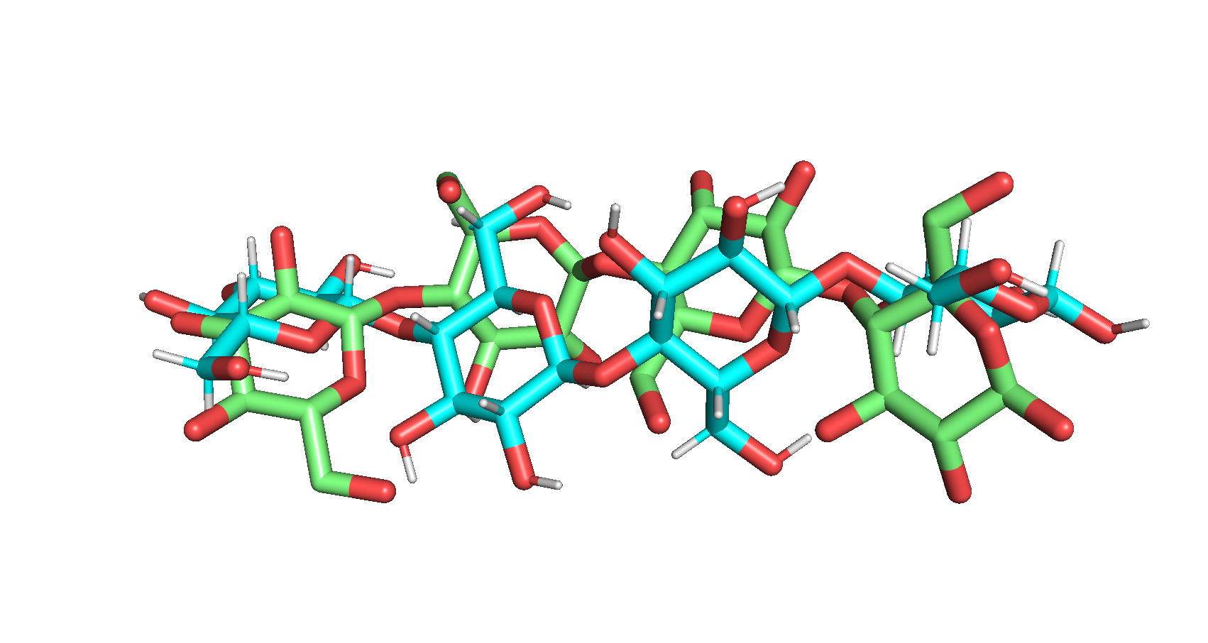
Now we can compare the ensemble of glycan conformations with the reference structure. To do this, we will superimpose the two structures and calculate the RMSD.
File menu -> Open -> select 1UU6_l_u_ens
Let us split the ensemble in its constituent models:
Now we can calculate the RMSD of each conformation in the ensemble:
align 1UU6_l_u_ens_0001, 1UU6, cycles=0
Repeat this command for each member of the ensemble.
Is at least one of these models closer to the bound structure than the original GLYCAM conformation?
Docking from an ensemble of glycan conformations
In a previous BONUS section we described how to generate an ensemble of glycan conformations using a short MD refinement protocol. We can now use this ensemble to dock the protein to multiple glycan conformations.
To do this, we will use the protein-glycan-ens.cfg, available in the haddock3 directory of the archive you downloaded.
Besides the presence of the glycan ensemble (1UU6_l_u_ens) in place of the single structure (1UU6_l_u), the only difference
between this protocol and the previous one is the sampling parameter at
the rigidbody docking level: as multiple conformations are being docked, in order to sample each starting conformation a sufficient amount of time we increase the number of models generated:
...
run_dir = "run_prot-gly_ensemble"

# list, insert full path
molecules = [
    "../pdbs/1OLR_clean.pdb",
    "../pdbs/1UU6_l_u_ens.pdb",
]

[topoaa]

[rigidbody]
ambig_fname = "../restraints/ambig.tbl"
w_vdw = 1
sampling = 4000

[caprieval]
reference_fname = "../pdbs/1UU6_target.pdb"
...Such information would not be available in a realistic modelling scenario, as the bound structure (1UU6 here) would be unknown.
BONUS2: Modifying the scoring weights at the flexible refinement stage
In the HADDOCK3 configuration file we have used in this tutorial, the scoring weights for the flexible refinement stage are set to the default values. Thes can be found here.
Glycans are quite hydrophobic molecules and, in a protein-glycan complex, the van der Waals energy is typically playing a more important role than the electrostatic interactions. We can therefore try to decrease the weight of the electrostatic energy term at the flexible refinement stage.
To do this, we need to modify the configuration file. The relevant section is the flexref module:
[flexref]
ambig_fname = "../restraints/ambig.tbl"
tolerance = 5
w_elec = 0.4
Setting w_elec to 0.4 (in place of 1.0) will downscale the electrostatic weight by a factor of 2.5.
You can now try to run the docking again with this new configuration file. You can either do this by running the modified configuration file (protein-glycan-elec.cfg, always from the haddock3 directory):
haddock3 protein-glycan-elec.cfg
or by restarting the existing run upon modifying the protein-glycan.cfg file:
haddock3 protein-glycan.cfg --restart 7
This will restart the run from the flexible refinement stage, using the new scoring weights.
Repeat the analysis performed in the previous sections to evaluate the quality of the docking models
What is the impact of the change in the scoring weights on the ranking of the models?