Welcome to the Haddock3 user manual
HADDOCK, standing for High Ambiguity Driven protein-protein DOCKing, is a widely used computational tool for the integrative modeling of biomolecular interactions. Developed by researchers at Utrecht University in the BonvinLab for more than 20 years, it integrates various types of experimental data, biochemical, biophysical, bioinformatic prediction, and knowledge to guide the docking process.
In this manual, we will describe:
- the basic concepts of HADDOCK
- the new functionalities of the haddock3 software suite
- how to create custom workflows
- provide example workflows
Navigate through the manual
On the top-left part of your screen, you will find three icons:
- stacked lines: allows to display/hide the table of content
- brushes: allows to tune the colors of the manual
- the magnifying glass: perform keyword text search in the entire manual and access corresponding pages

HADDOCK - High Ambiguity Driven Docking
High Ambiguity Driven DOCKing (HADDOCK), is now a long standing docking software, that harness the power of CNS (Crystallography and NMR System – https://cns-online.org) for structure calculation of molecular complexes. What distinguishes HADDOCK from other docking software is its ability, inherited from CNS, to incorporate experimental data as restraints and use these to guide the docking process alongside traditional energetics and shape complementarity. Moreover, the intimate coupling with CNS endows HADDOCK with the ability to actually produce models of sufficient quality to be archived in the Protein Data Bank.
A central aspect of HADDOCK is the definition of Ambiguous Interaction Restraints or AIRs. These allow the translation of raw data such as NMR chemical shift perturbation or mutagenesis experiments into distance restraints that are incorporated into the energy function used in the calculations. AIRs are defined through a list of residues that fall under two categories: active and passive. Generally, active residues are those of central importance for the interaction, such as residues whose knockouts abolish the interaction or those where the chemical shift perturbation is higher. Throughout the simulation, these active residues are restrained to be part of the interface, if possible, otherwise incurring a scoring penalty. Passive residues are those that contribute to the interaction but are deemed of less importance. If such a residue does not belong in the interface there is no scoring penalty. Hence, a careful selection of which residues are active and which are passive is critical for the success of the docking.
HADDOCK scoring function
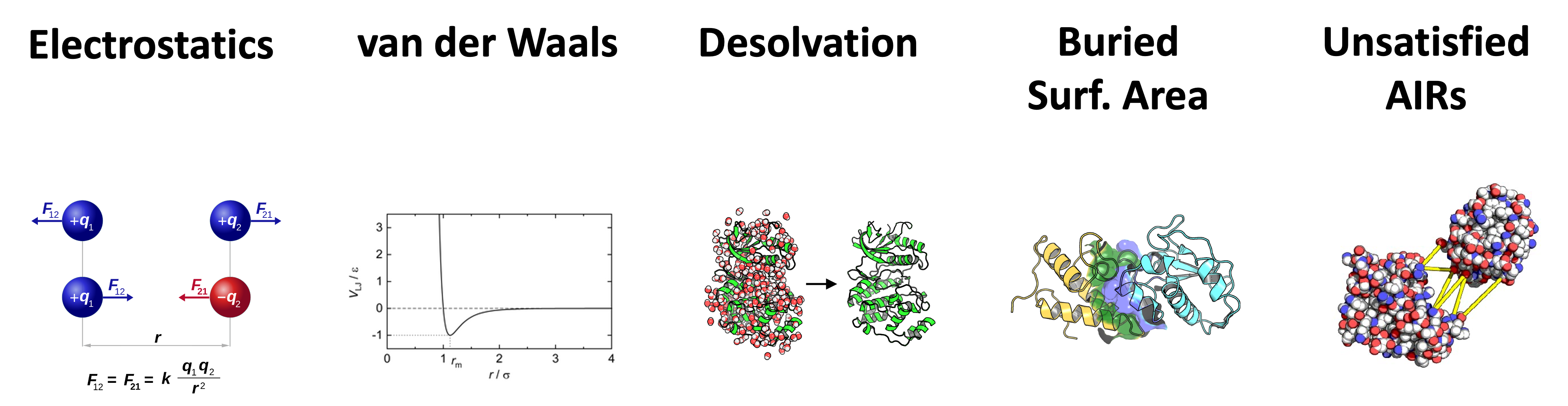
CNS modules use the HADDOCK scoring function to score and rank generated models. The HADDOCK scoring function consists of a linear combination of various weighted physics-based energy terms and buried surface area.
The scoring is performed according to the weighted sum (HADDOCK score) of the 6 following terms:
- Eelec: electrostatic intermolecular energy
- Evdw: van der Waals intermolecular energy
- Edesol: desolvation energy
- BSA: buried surface area
- Eair: distance restraints energy (only unambiguous and AIR (ambig) restraints)
- Esym: symmetry restraints energy (NCS and C2/C3/C5 terms)
As the weights for each of the scoring function components differs for the various available CNS module, they will be described in each of the modules (see: haddock3 modules).
Of course, these weights can be tuned by the user, by modifying their related parameters:
w_elec: to tune the electrostatic intermolecular energy weightw_vdw: to tune the van der Waals intermolecular energy weightw_desolv: to tune the desolvation energy weightw_bsa: to tune the buried surface area weightw_air: to tune the distance restraints energy (only unambiguous and AIR (ambig) restraints) weightw_sym: to tune the symmetry restraints energy (NCS and C2/C3/C5 terms) weight
Haddock3
Haddock3 is the next-generation integrative modeling software of the long-lasting HADDOCK docking tool. It represents a complete rethinking and rewriting of the HADDOCK2.X series, implementing a new way to interact with HADDOCK and offering new features to users who can now define custom workflows.
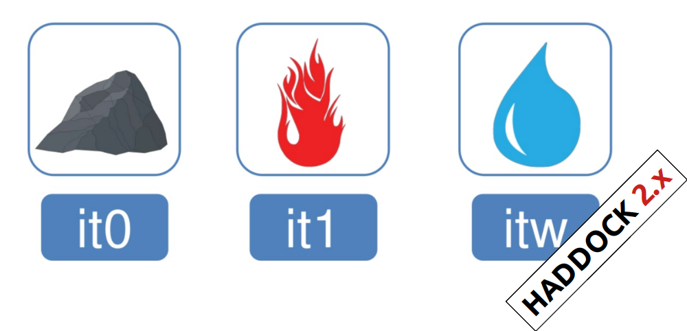
In the previous HADDOCK2.x versions, users had access to a highly parameterisable yet rigid simulation pipeline composed of three steps: rigid-body docking (it0), semi-flexible refinement (it1), and final refinement (itw).
In HADDOCK3, users have the freedom to configure docking workflows into functional pipelines by combining the different HADDOCK3 modules, thus adapting the workflows to their projects. HADDOCK3 has therefore developed to truthfully work like a puzzle of many pieces (simulation modules) that users can combine freely. To this end, the “old” HADDOCK machinery has been modularized, and several new modules added, including third-party software additions. As a result, the modularization achieved in HADDOCK3 allows users to duplicate steps within one workflow (e.g., to repeat twice the it1 stage of the HADDOCK2.x rigid workflow).
Note that, for simplification purposes, at this time, not all functionalities of HADDOCK2.x have been ported to HADDOCK3, which does not (yet) support NMR RDC, PCS and diffusion anisotropy restraints, cryo-EM restraints and coarse-graining. Any type of information that can be converted into ambiguous interaction restraints can, however, be used in HADDOCK3, which also supports the ab initio docking modes of HADDOCK.
To keep HADDOCK3 modules organized, we cataloged them into several categories. However, there are no constraints on piping modules of different categories.
The main module categories are “topology”, “sampling”, “refinement”, “scoring”, and “analysis”. There is no limit to how many modules can belong to a category. Modules are added as developed, and new categories will be created if/when needed. You can access the HADDOCK3 documentation page, or read the user manual for the list of all categories and modules.
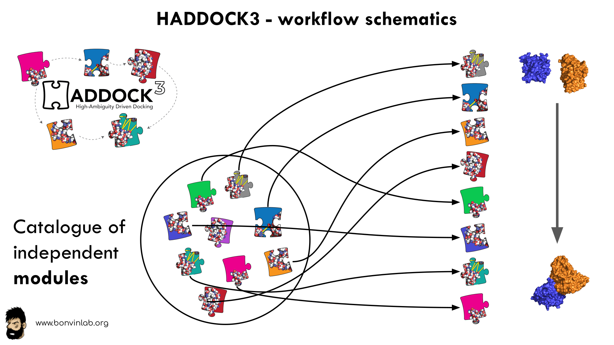
The HADDOCK3 workflows are defined in simple configuration text files, similar to the TOML format but with extra features. Contrary to HADDOCK2.X which follows a rigid (yet highly parameterisable) procedure, in HADDOCK3, you can create your own simulation workflows by combining a multitude of independent modules that perform specialized tasks. Details on how to create a workflow is provided in a dedicated section. We also provide a set of docking scenario examples, containing quite a variety of different protocols that can also guide you.
How to install haddock3
To install haddock3, you will need to sucessfully manage to get your hands on the following four steps:
A complete guide is also available on our haddock3 GitHub repository.
You can also install HADDOCK3 using docker
Virtual environments
Haddock3 makes use of system variables as well as external libraries.
To ensure a reproducible and stable functional version of haddock3, we strongly advise to intall it using a virual environment.
When used from within a virtual environment, common installation tools such as pip will install Python packages into a virtual environment, limiting conflicts with other tools already installed on your computing engine.
Two major environments managing system are effective and capable of installing haddock3, namely venv and conda/mini-conda. Below you will find the instructions on how to install them and set up a proper haddock3 environment.
venv
As the venv library is part of the python3 standard library, hence there is no need to install it, considering python3 is installed on your machine.
By using venv, you will be able to set the python3 version you want (>=3.9 for haddock3).
For more details and troubleshooting with the venv library, have a look at its documentation
Then create a new clean environment with the following command:
python3.9 -m venv .haddock3-env
# or
python3.10 -m venv .haddock3-env
# or
python3.11 -m venv .haddock3-env
# or
python3.12 -m venv .haddock3-env
Finally, you should activate the environment, and you are ready for the next steps
source .haddock3-env/bin/activate
Anaconda / miniconda
For more details and troubleshooting with the conda library, have a look at its documentation
Then create a new haddock3-env environment with the following command:
conda create -n haddock3-env python=3.9
# or
conda create -n haddock3-env python=3.10
# or
conda create -n haddock3-env python=3.11
# or
conda create -n haddock3-env python=3.12
Finally, you should activate the environment, and you are ready for the next steps
conda activate haddock3-env
Install via the Python Package Index (PyPI)
We have simplified the installation of Haddock3 by adding it to the Python Package Index.
Therefore, the only command you should run is the following:
# Activate your haddock3 virtual env
# ...
# run pip install haddock3
pip install haddock3
Note that by running pip install haddock3, you will be able to use haddock3, but the examples will not be provided.
To obtain them, you should install haddock3 from the source code (as described below).
DISCLAMER: By running this command, you will download a compiled executable of CNS (Crystallographic and NMR System) which is free of use for non-profit applications. For commercial use, it is your own responsibility to have a proper license. For details refer to the DISCLAIMER file in the HADDOCK3 repository.
Download haddock3 source code
Haddock3 is an open source software and therefore its source code can be downloaded at any time. We are hosting the code on a dedicated GitHub repository, allowing for better version control, code development and maintainability.
For usage tracking purposes (to avoid counting robots downloading the tool), we advise users to download it from our lab page, as it eases the reporting tasks to authorities supporting the development of this project with grants.
To install haddock3 from the source, we suggest running the following commands:
# First, download the source code:
git clone https://github.com/haddocking/haddock3.git
cd haddock3

# Setup the virtural environnement:
python3.9 -m venv .haddock3-env
source .haddock3-env/bin/activate

# Install haddock3
pip install .
# DISCLAMER
# By running this command, you will download a compiled executable
# of CNS (Crystallographic and NMR System) which is free of use
# for non-profit applications.
# For commercial use it is your own responsibility to have a proper license.
# For details refer to the DISCLAIMER file in the HADDOCK3 repository.
# here -> https://github.com/haddocking/haddock3/blob/main/DISCLAIMER.md
Development version
To install the development version of haddock3, you should add extra arguments to the pip install commands, so other libraries will be downloaded too:
# First, download the source code:
git clone https://github.com/haddocking/haddock3.git
cd haddock3

# Setup the virtural environnement:
python3.9 -m venv .haddock3-env
source .haddock3-env/bin/activate

# Install haddock3
pip install -e '.[dev,docs]'
A complete guide on how to setup an adequate development environment can be found here: DEVELOPMENT.md
Install CNS
HADDOCK is using Crystallography & NMR System (CNS) as a core computing engine. CNS is a FORTRAN66 code that must be compiled on your machine, for your own hardware.
Pre-compiled binaries
To simplify the installation procedure of haddock3, we now provide pre-compiled CNS binaries, that are automatically installed when you run pip install haddock3.
Therefore there should be no need of compiling it yourself, which was one of the major issue related to the installation of HADDOCK.
DISCLAMER: By running this command, you will download a compiled executable of CNS (Crystallographic and NMR System) which is free of use for non-profit applications. For commercial use, it is your own responsibility to have a proper license. For details refer to the DISCLAIMER file in the HADDOCK3 repository.
Compiling CNS on your own
Please see the up-to-date installation procedure of CNS here, where you will find specific guides and troubleshooting sections.
Once compiled, you need to replace the executable located in the haddock package in virtual environnement (haddock/bin/).
Here is an example:
# Given you have created a virtual env named .haddock3-env
python3.12 -m venv .haddock3-env
# and already installed haddock3
pip install .
# You can replace the cns executable by your own newly generated executable in the site-packages/haddock/bin/ directory
cp my-own-cns-executable .haddock3-env/lib/python3.12/site-packages/haddock/bin/cns
Using HADDOCK3 through its docker image
As part of the possible usage of HADDOCK3, we also provide a ready to use docker image of HADDOCK3, where tools and packages are already installed.
Note that this image corresponds to the latest release of HADDOCK3, and not the latest version. To use the latest version in docker rather build it directly (see below).
DOCKER
To be able to use a provided image, you first need to have docker installed.
Please follow the instructions you can find there: https://www.docker.com/.
Installing HADDOCK3 from provided images
Installing the latest release
docker pull ghcr.io/haddocking/haddock3:latest
docker tag ghcr.io/haddocking/haddock3:latest haddock3
Install a specific version
To install a specific version of haddock3, you must specify which release you are interested in (e.g.: 2025.05.0)
docker run ghcr.io/haddocking/haddock3:2025.05.0
docker tag ghcr.io/haddocking/haddock3:2025.05.0 haddock3
Check here to see the list of available releases.
Building your own docker container from the latest version of HADDOCK3
With this approach, you will be building a new docker image from the latest version available in the main branch of the haddock3 GitHub repository.
# Build a container from the latest haddock3 version
git clone https://github.com/haddocking/haddock3.git
cd haddock3
docker build . --label haddock3 --tag haddock3
Run HADDOCK with a workflow file, e.g. myworkflow.cfg
docker run \
    -v $(pwd):/cwd  \
    --workdir /cwd \
    -u $(id -u)  \
    haddock3 \
    myworkflow.cfg
Command line interfaces
Haddock3 is a software that can read configuration files and compute data. While there will be a web application, haddock3 does not have a graphical user interface and must used from the command line. While this may have some negative impact for some inexperienced users, it is also very powerful as it allows custom scripting to launch haddock3, and therefore integrating it in your own pipelines is easier.
To use the command line interface, you must open a terminal:
- [iTerm / Terminal]: for Mac users, default terminals are available and fully functional.
- [WindowsPowerShell]: The Windows solution to open a terminal.
- VSCode: an integrated developing environment (IDE) that allows you to run command lines in the terminal.
Haddock3 comes with several Command Line Interfaces (CLIs), that are described and listed below:
- haddock3: Main CLI for running a workflow.
- haddock3-cfg: Obtain information about module parameters
- haddock3-restraints: Generation of restraints.
- haddock-restraints: Generation of restraints with the standalone application
- haddock3-score: Scoring CLI.
- haddock3-analyse: Analysis of output.
- haddock3-traceback: Traceback of generated docking models.
- haddock3-re: Recomputing modules with different parameters.
- haddock3-re score: To modify scoring function weights.
- haddock3-re clustfcc: To modify
[clustfcc]parameters. - haddock3-re clustrmsd: To modify
[clustrmsd]parameters.
- haddock3-copy: To copy a haddock3 run.
- haddock3-clean: Archiving a run.
- haddock3-unpack: Uncompressing an archived a run.
- haddock3-pp: Pre-processing of input files.
haddock3
The main command line, haddock3 is used to launch a Haddock3 workflow from a configuration file.
It takes a positional argument, the path to the configuration file.
haddock3 workflow.cfg
Also, two optional arguments can be used:
--restart <module_id>: allows to restart the workflow restarting for the module id. Note that previously generated folders from the selected step onward will be deleted.--extend-run <run_directory>: allows to start the new workflow from the last step of a previously computed run.
haddock3-cfg
Another very interesting CLI is haddock3-cfg.
This CLI allows you to list the parameter names, their description, and default values for each available module.
Used without any option, the command haddock3-cfg will return all Global parameters.
To access the list of parameters for a given module, you should use the optional argument -m <module_name>.
As an example, to list available parameters for the module seletopclusts, you should run the following command:
haddock3-cfg -m seletopclusts
Please note that all the parameters for each module are also available in the online documentation.
haddock3-restraints
The CLI haddock3-restraints is made to generate restraints used either as ambiguous restraints or unambiguous ones.
The haddock3-restraints CLI is composed of several sub-commands, each one dedicated to some specific actions, such as:
- Searching for solvent-accessible residues
- Gathering neighbors of a selection
- Maintaining the conformation of a single chain with a potential gap
- Generating ambiguous restraints from active and passive residues
- Generating planes and corresponding restraints
As this CLI is more specialized, we have made a special chapter in this manual to explain all the functionalities.
haddock-restraints
The CLI haddock-restraints has its own documentation, please see: bonvinlab.org/haddock-restraints and also the online interface at wenmr.science.uu.nl/haddock-restraints
It is composed of subcommands and can generate simple and complex restraints files. You define active/passive residues and can filter residues that are buried, define passive residues around the active ones, keep molecules together during docking (or keep a ligand in place), define "true-interface" restraints, list residues that are in the interface, define z-coordinate restraints (useful for membranes) and also generate unambigous restraints - a more strict type of true interface restraints.
By passing the --pml argument you can also generate a PyMol script for easy visualization of the restraints.
haddock3-score
The haddock3-score is a CLI made for scoring a single complex.
The topologies are created and a small energy minimization is performed on the complex before the evaluation of the haddock score components.
It is dedicated to the scoring of it and only returns the computed haddock score and its components.
It is a shortcut to a full configuration file that would contain the topoaa and emscoring modules.
To use it, provide the path to the complex to be scored:
haddock3-score path/to/complex.pdb
This CLI can take optional parameters using the -p flag, where the user can provide the set of parameters and values to tune the weights of the Haddock scoring function.
Be aware that only parameters available for the emscoring module are accepted.
To tune the haddock3 scoring function weights, there are basically only 5 parameters to be tuned.
- w_vdw: to tune the weight of the Van der Waals term
- w_elec: to tune the weight of the Electrostatic term
- w_desolv: to tune the weight of the Desolvation term
- w_air: to tune the weight of the Ambiguous Restraints term
- w_bsa: to tune the weight of the Buried Surface Area term
Note that, if a parameter is not tuned, the default scoring function weights are used.
As an example, this command would tune the Van der Waals term during the evaluation of the complex:
haddock3-score path/to/complex.pdb -p w_vdw 0.5
Note how the parameter name and its new value are separated by a space.
To modify multiple parameters, just add the new parameter separated by a space:
haddock3-score path/to/complex.pdb -p w_vdw 0.5 w_bsa 0.2
haddock3-analyse
Haddock3 contains functionalities that allow the analysis of various steps of the workflow, even after it has been completed. The haddock3-analyse command is the main tool for the analysis of one or more workflow steps. Typically it runs automatically at the end of a HADDOCK3 workflow (activated by the postprocess option), but it can be run independently as well.
haddock3-analyse -r my-run-folder -m 2 5 6
Here my-run-folder is the run directory and 2, 5, and 6 are the steps that you want to analyze.
The command will inspect the folder, looking for the existing models. If the selected module is a caprieval module, haddock3-analyse simply loads the capri_ss.tsv and capri_clt.tsv files
produced by the caprieval module. Otherwise, haddock3-analyse runs a caprieval analysis of the models.
You can provide some caprieval-specific parameters
using the following syntax:
haddock3-analyse -r my-run-folder -m 2 5 6 -p reference_fname my_ref.pdb receptor_chain F
Here the -p key tells the code that you are about to insert [caprieval] parameters, whose name should match the parameter name of the module. Each parameter name and the corresponding value must be separated by a space character.
Another parameter that can be specified is top_clusters, which defines how many of the first N clusters will be considered in the analysis.
This value is set to 10 by default.
haddock3-analyse -r my-run-folder -m 2 5 6 --top_clusters 12
This number is meaningless when dealing with models with no cluster information, that is, models that have never been clustered before.
By default haddock3-analyse produces plotly plots in the HTML format, but the user can select
one of the formats available here,
while also adjusting the resolution with the scale parameter:
haddock3-analyse -r my-run-folder -m 2 5 6 --format pdf --scale 2.0
The analysis folder
After running haddock3-analyse you can check the content of the analysis directory in your run folder.
If everything went successfully, one of the above commands should have produced an analysis folder structured as
my-run-folder/
|--- analysis/
 |--- 2_caprieval_analysis
 |--- 5_seletopclusts_analysis
 |--- 6_flexref_analysis
Each subfolder contains all the analysis plots related to that specific step of the workflow.
By default haddock3-analyse produces a set of scatter plots that compare each HADDOCK energy term
(i.e., the HADDOCK score and its components) to the different metrics used to evaluate the quality of a model,
such as the interface-RMSD, Fnat, DOCKQ, and so on. An example is available here.
For each of the energy components and the metrics mentioned above haddock3-analyse produces also a box plot, in which each cluster
is considered separately. An example is available here.
The report
Scatter plots, box plots, CAPRI statistics, and interactive visualization of the models are available in the report.html file, present
in each analysis subfolder. In order to visualize the models it is necessary to start a local server at the end of the haddock3-analyse run,
following the indications provided in the log file:
[2023-08-24 10:09:09,552 cli_analyse INFO] View the results in analysis/12_caprieval_analysis/report.html
[2023-08-24 10:09:09,552 cli_analyse INFO] To view structures or download the structure files, in a terminal run the command
`python -m http.server --directory /haddock3/examples/docking-antibody-antigen/run1-CDR-acc-cltsel-test`.
By default, http server runs on `http://0.0.0.0:8000/`. Open the link
http://0.0.0.0:8000/analysis/12_caprieval_analysis/report.html in a web browser.
Launch this command to open the report:
python -m http.server --directory path-to-my-run
In the browser, you can navigate to each analysis subfolder and open the report.html file. If you are not interested in
visualizing the models, you can simply open the report.html file in a standard browser. An example report can be visualized here.
haddock3-traceback
HADDOCK3 is highly customizable and modular, as the user can introduce several refinement, clustering, and scoring steps in a workflow.
Quantifying the impact of the different modules is important while developing a novel docking protocol. The haddock3-traceback command
is developed to assist the user in this task, as it allows to "connect" all the models generated in a HADDOCK3 workflow:
haddock3-traceback my-run-folder
haddock3-traceback creates a traceback subfolder within the my-run-folder directory, containing a traceback.tsv table:
00_topo1     00_topo2        01_rigidbody            01_rigidbody_rank       04_seletopclusts        04_seletopclusts_rank   06_flexref      06_flexref_rank
4G6K.psf     4I1B.psf        rigidbody_10.pdb        3                       cluster_1_model_1.pdb   1                       flexref_1.pdb   2
4G6K.psf     4I1B.psf        rigidbody_11.pdb        10                      cluster_1_model_2.pdb   3                       flexref_3.pdb   1
4G6K.psf     4I1B.psf        rigidbody_18.pdb        4                       cluster_2_model_1.pdb   2                       flexref_2.pdb   4
4G6K.psf     4I1B.psf        rigidbody_20.pdb        15                      cluster_2_model_2.pdb   4                       flexref_4.pdb   3
In this table, each row represents a model that has been produced by the workflow.
The (typically) two used topologies are reported first,
and then each module has its own column, containing the name and rank of the model at that stage.
As an example, in the first row of the
table above rigidbody_10.pdb is ranked 3rd at the rigidbody stage.
Then, it becomes cluster_1_model_1.pdb (ranked 1st) after
the seletopclusts module.
This model is then refined in flexref_1.pdb, which turns out to be the 2nd best model at the end of the workflow.
The table can be easily parsed and used to evaluate the impact of different refinement steps on the different models.
The postprocess option
You may want to run the haddock3-analyse and haddock3-traceback commands by default at the end of the workflow.
The postprocess option of a standard HADDOCK3 configuration (.cfg) file is devoted to this task. At first, it forces HADDOCK3
to execute haddock3-analyse on all the XX_caprieval folders found in the workflow, therefore loading data present in the CAPRI tables.
Second, it executes the haddock3-traceback command.
By default, postprocess is set to true but can also be de-activated at the beginning of your configuration file:
 ====================================================================
# This is a HADDOCK3 configuration file

# directory in which the docking will be done
run_dir = "my-run-folder"

# postprocess the run
postprocess = false

...
Note: If speed is an issue, please turn the postprocess option off for your run!
You can find additional help by running the command: haddock3-analyse -h and haddock3-traceback -h and reading
the parameters' explanations. Otherwise, ask us in the "issues" forum.
haddock3-re
The haddock3-re CLI is dedicated to recomputing some steps in your workflow.
This can be very useful as it allows us to fine-tune parameters and evaluate the impact on the results.
haddock3-re takes two mandatory positional arguments:
- **1:**The name of the subcommand
- **2:**Path to the module on which to apply the modifications in your run
By running haddock3-re, a new directory will be created, with the _interactive suffix, where the new results are stored.
Relaunching several times haddock3-re on the same directory will update the content in the _interactive one.
For now, three modules can be recomputed and tuned, [caprieval], [clustfcc] and [clustrmsd].
-re score
The subcommand haddock3-re score, allows to tune the weights of the HADDOCK scoring function.
It takes a [caprieval] step folder as positional argument and the tuned weights for the scoring function.
Note that if you do not provide new weights as optional arguments, previous weights used in the run are used.
Usage:
haddock3-re clustrmsd <path/to/the/module/step/X_caprieval>

optional arguments:
  -e W_ELEC, --w_elec W_ELEC
                        weight of the electrostatic component.
  -w W_VDW, --w_vdw W_VDW
                        weight of the van-der-Waals component.
  -d W_DESOLV, --w_desolv W_DESOLV
                        weight of the desolvation component.
  -b W_BSA, --w_bsa W_BSA
                        weight of the BSA component.
  -a W_AIR, --w_air W_AIR
                        weight of the AIR component.
-re clustfcc
The subcommand haddock3-re clustfcc, allows to tune the clustering parameters of the [clustfcc] module.
It takes a [clustfcc] step folder as a positional argument and the tuned parameters for the module.
Note that if you do not provide new parameters as optional arguments, previous ones will be used instead.
Usage:
haddock3-re clustfcc <path/to/the/module/step/X_clustfcc>

optional arguments:
  -f CLUST_CUTOFF, --clust_cutoff CLUST_CUTOFF
                        Minimum fraction of common contacts to be considered in a cluster.
  -s STRICTNESS, --strictness STRICTNESS
                        Strictness factor.
  -t MIN_POPULATION, --min_population MIN_POPULATION
                        Clustering population threshold.
  -p, --plot_matrix     Generate the matrix plot with the clusters.
-re clustrmsd
The subcommand haddock3-re clustrmsd, allows to tune the clustering parameters of the [clustrmsd] module.
It takes a [clustrmsd] step folder as a positional argument, and the tuned parameters for the module.
Note that if you do not provide new parameters as optional arguments, previous ones will be used instead.
Usage:
haddock3-re clustrmsd <path/to/the/module/step/X_clustrmsd>

optional arguments:
  -n N_CLUSTERS, --n_clusters N_CLUSTERS
                        number of clusters to generate.
  -d CLUST_CUTOFF, --clust_cutoff CLUST_CUTOFF
                        clustering cutoff distance.
  -t MIN_POPULATION, --min_population MIN_POPULATION
                        minimum cluster population.
  -p, --plot_matrix     Generate the matrix plot with the clusters.
Please note that parameters --n_clusters (defining the number of clusters you want)
and --clust_cutoff are mutually exclusive,
as the former is cutting the dendrogram at a height satisfying the number of desired clusters
while the latter is cutting the dendrogram at the --clust_cutoff value height.
haddock3-copy
The haddock3-copy CLI allows one to copy the content of a run to another run directory.
It takes three arguments:
-r run_directoryis the directory of a previously computed haddock3 run.-o new_run_directoryis the new directory where to make to copy of the old run.-m module_id_X module_id_Yis the list of modules you wish to copy (separated by spaces).
As an example, consider your previous run directory is named run1 and contains the following modules:
run1/
  0_topoaa/
  1_rigidbody/
  2_caprieval/
  3_seletop/
  4_flexref/
 (etc...)
You may want to use 4_flexref step folder as a starting point for a new run named run2.
To do so, run the following command:
haddock3-copy -r run1 -m 0 4 -o run2
Notes:
- the flag
-mallows to define which modules must be copied, and modules0(for0_topoaa) and4(for4_flexref) are space separated. - in this case, we also copy the content of
0_topoaa, this is because topologies are stored in this module directory, and we must have access to them if we are using another module requiring CNS topology to run. - it is often recommended to always copy the
topoaadirectory, as we will often require the topologies later in the workflow.
WARNING:
To copy the content of a run and modify the paths, we are using the sed command, searching to replace the previous run directory name (run1) with the new one (run2) in all the generated files to make sure that paths will be functional in the new run directory.
In some cases, this can lead to some artifacts, such as the modification of attribute names if your run directory contains a name that is used by haddock3.
Here is a list of run directory names NOT to use:
- topology
- score
- emref
- etc...
The best solution is to always use a unique name that describes the content of the run.
haddock3-clean
Thehaddock3-clean CLI performs file archiving and file compressing operations on the output of a haddock3 run directory.
This CLI can save you some hard drive storage space, as the multiple files generated by HADDOCK can lead to several gigabytes of data, therefore compressing them allows you to keep them while saving some precious place.
All .inp and .out files are deleted except for the first one, which is compressed to .gz.
On the other hand, all .seed and .con files are compressed and archived into .tgz files.
Finally, .pdb and .psf files are compressed to .gz.
The <run_directory> can either be a whole HADDOCK3 run folder or a specific folder of the workflow step.
Please note that by default this CLI is launched automatically at the end of a workflow.
It is exposed as a general parameter clean = true.
To switch off this behavior, you can set it to false in your configuration file.
Usages:
# Display help
haddock3-clean -h
haddock3-clean run1 # Where run1 is a path to a haddock3 run directory
haddock3-clean run1/1_rigidbody  # Where 1_rigidbody is the output of the rigidbody module
haddock3-clean run1 -n  # uses all cores
haddock3-clean run1 -n 2  # uses 2 cores
Here is the list of arguments:
positional arguments:
  run_dir               The run directory.

optional arguments:
  -n [NCORES], --ncores [NCORES]
                        The number of threads to use. Uses 1 if not specified. Uses all available threads if `-n` is given. Else,
                        uses the number indicated, for example: `-n 4` will use 4 threads.
  -v, --version         show version
haddock3-unpack
The haddock3-unpack CLI is the opposite of the haddock3-clean one.
It takes a haddock3 run directory as input (or the output directory of a module), and uncompresses any archived file.
This CLI can be especially useful when your run has been archived, but you would like to open a PDB file using a molecular viewer.
The unpacking process performs file unpacking and file decompressing operations.
Files with extensions seed and con are unpacked from their .tgz files.
While files with .pdb.gz and .psf.gz extensions are uncompressed.
If --all is given, unpack also .inp.gz and .out.gz files.
Usage:
# To display help
haddock3-unpack -h
# To unpack the entire run directory
haddock3-unpack run1
# To unpack the output directory of a specific module
haddock3-unpack run1/1_rigidbody
# Define the number of cores to use
haddock3-unpack run1 -n  # uses all cores
haddock3-unpack run1 -n 2  # uses 2 cores
# Add the -a or --all to specify that all compressed files must be unpacked
haddock3-unpack run1 -n 2 -a
haddock3-unpack run1 -n 2 --all
Arguments:
positional arguments:
  run_dir               The run directory.

optional arguments:
  -h, --help            show this help message and exit
  --all, -a             Unpack all files (including `.inp` and `.out`).
  -n [NCORES], --ncores [NCORES]
                        The number of threads to use. Uses 1 if not specified. Uses all available threads if `-n` is given. Else,
                        uses the number indicated, for example: `-n 4` will use 4 threads.
  -v, --version         show version
haddock3-pp
The haddock3-pp is a pre-processing (-pp) CLI, dedicated to processing PDB files for agreement with HADDOCK3 requirements.
You can use the --dry option to report on the performed changes without actually performing the changes.
Corrected PDBs are saved to new files named after the --suffix option.
Original PDBs are never overwritten unless the --suffix is given an empty string.
You can pass multiple PDB files to the command line.
Usage:
haddock-pp file1.pdb file2.pdb
haddock-pp file1.pdb file2.pdb --suffix _new
haddock-pp file1.pdb file2.pdb --dry
Arguments:
positional arguments:
  pdb_files             Input PDB files.

options:
  -h, --help            show this help message and exit
  -d, --dry             Perform a dry run. Informs changes without modifying files.
  -t [TOPFILE ...], --topfile [TOPFILE ...]
                        Additional .top files.
  -s SUFFIX, --suffix SUFFIX
                        Suffix to output files. Defaults to '_processed'
  -odir OUTPUT_DIRECTORY, --output-directory OUTPUT_DIRECTORY
                        The directory where to save the output.
Input files
Over the years, HADDOCK was updated to increase the range of biomolecular entities to deal with. Currently, we support a broad range of molecular types, such as protein, DNA, RNA, glycans, cyclic-peptides and small-molecules. In addition, several modified residues/nucleotides are also available. For the full list of supported molecules, please refer to https://wenmr.science.uu.nl/haddock2.4/library. If you wish to work with a molecule type that is not present in this list, please refer to the Dealing with non-standard molecules section.
In the following sections, we will tackle the variety and specificity of each of the molecule types.
Supported file format
Haddock3 currently supports files in PDB and mmCIF format. The PDB format is quite strict, and all characters must be well positioned in the file.
To make sure your file is correctly formatted, you can use the pdbtools library (which should be already installed in your haddock3-env virtual environment),
or read this online resource where it is well explained.
Please refer to the pdb-tools section for more information on how to use it.
PDB format
In order to run HADDOCK you need to have the structures of the molecules (or fragments thereof) in PDB format. There are a few points to pay attention to when preparing the PDBs for HADDOCK.
-
Make sure that all PDB files end with an END statement
-
If providing a conformational ensemble (e.g.: from an NMR PDB entry, or out of a MD simulation), each model should start with a MODEL statement and end with an ENDMDL statement and the file should terminate with a END.
-
haddock3 will not check for breaks in the chain (e.g. missing density in crystal structures or between the two strands of a DNA molecules). In the case of multiple chains within one molecule (e.g. DNA) or in the presence of co-factors, it is recommended to add a TER statement in between the chains/sub-molecules. Also, consider using the
haddock3-restraints restrain_bodiescommand line to generate restraints and input them as unambiguous restraints using theunambig_fnameparameter. -
If your input molecule consists of multiple chains with overlapping numbering you will have to renumber those (or shift the numbering of some parts) in order to avoid overlapping numbering. HADDOCK will treat each molecule with a single chainID and overlap in numbering will lead to problems.
-
Higher-resolution crystal structures often contain multiple occupancy side-chain conformations, which means one residue might have multiple conformations present in the crystal structure, each with a partial occupancy. The definition of alternative conformations is often reflected by the presence of a
AandBbefore the residue name for the atoms having multiple conformations. To avoid problems, only one conformation should be retained (the web server will raise an error for such cases). This can be easily done using our PDB-tools. Alternatively, you can also make use of our new PDB-tools webserver{:target="_blank"} for this. The script that allows you to remove double occupancies ispdb_selaltloc. Its default behavior is to only keep the first (A) conformation, but you can select other conformations if wanted. -
HADDOCK can deal with ions. You will have however to make sure that the ion naming is consistent with the ion topologies provided in HADDOCK. For example, a CA heteroatom with a residue name CA will be interpreted as a neutral calcium atom. A doubly charged calcium ion should be named CA+2 with CA2 as residue name to be properly recognized by HADDOCK. (See also the FAQ for docking in the presence of ions).
A list of supported modified amino acids and ions is available online.
Note: Most of the tasks mentioned above can also be performed using our PDB-tools python scripts (Rodrigues et al. F1000 Research (2018)) to manipulate PDB files, select and rename chains and segids, renumber residues... and much more! It should be installed by default in your haddock3 environment. And a dedicated section is present in this manual.
For more details, see for this our GitHub repository. Alternatively, you can also make use of our new PDB-tools webserver.
Number of input molecules
Haddock3 currently supports up to 20 separate input molecules, thus allowing multi-body (1 <= N <= 20) docking. Each input molecule can be composed of an ensemble of conformations, allowing to implicitly represent the conformational sampling. Input molecules can also be composed of multiple chains, allowing for their evaluation using scoring and analysis modules.
To input molecules, use the global parameter molecules = ["path/to/mol1.pdb", "path/to/mol2.pdb"].
Definition of a chain
A chain is defined by a letter in the 22nd position in the PDB file format.
Within the same file, two chains must be separated by a TER statement.
Do not worry if you have gaps (missing resiudes) in your chain, it will be automatically detected by HADDOCK.
To make sure the structure do not fall appart during molecular dynamics steps, you can add body-restraints ensuring the constant distance originally observed in the input file.
Conformational ensemble
Conformational ensembles are detected using the MODEL and ENDMDL keywords in the PDB file.
Note that if in your ensemble, we detect two types of REMARK statements when providing an ensemble:
REMARK MODEL X FROM conformationX.pdb: as generated bypdb_mkensemble, we will keep track of the origin of the conformation.REMARK X MODEL Y MD5 XXXXXXXXXXXXXXXXXX: as provided by CAPRI scoring set, we will keep track of the MD5 checksum of the input conformation/model.
Dealing with non-standard molecules
If you wish to work with a molecule type that is not present in the list of supported molecules, do not worry, as you will still be able to use HADDOCK. To properly function, HADDOCK requires to have access to the topology and parameters of a molecule to run the molecular dynamics protocols. The force field must therefore be updated by user-provided topology and parameter files.
In modules that use CNS, you can provide such files with the ligand_top_fname (for ligand topology filename) and ligand_param_fname (for ligand parameters filename) parameters, specifying the location where to find those two files.
How to generate topology and parameters for my ligand
Generating topology and parameters for your ligand is not trivial.
For this, you will need to use dedicated tools, such as acpype or ccp4-prodrg, or dedicated libraries such as BioBB.
Here are some useful resources on how to generate those:
- BioBB using acpype: The BioExcel BioBuildingBlock (BioBB) library is hosting several tutorials on how to perform computations with a variety of different tools. Here is a link to the workflow used to parametrize ligands: https://mmb.irbbarcelona.org/biobb/workflows/tutorials/biobb_wf_ligand_parameterization.
- Automated Topology Builder (ATB): Repository developed in Prof. Alan Mark's group at the University of Queensland in Brisbane: https://atb.uq.edu.au/.
- Using OpenBabel and acpype: A simple set of two commands can generate CNS ready topology and parameters using both OpenBabel and acpype.
# Install OpenBabel and acpype
pip install acpype==2023.10.27 openbabel-wheel==3.1.1.21
# First standardise and add hydrogens to your pdb file using OpenBabel
obabel -ipdb <input_file.pdb> -opdb -O ligand.pdb -h
# Use acpype to generate cns parameters and topology
acpype -i ligand.pdb -o cns -t -j -a ambe
PDB-Tools
PDB-tool is set of python scripts dedicated at manipulating PDB files, select and rename chains and segids, renumber residues... and much more! (Rodrigues et al. F1000 Research (2018)) The source code can be obtain from its GitHub repository. Alternatively you can also make use of our new PDB-tools webserver.
In addition, it comes as one of the dependencies installed by default in your haddock3 environement. Therefore, once the environement is activated, you will be able to access all the functionalities from the command line.
Here is a list of all available command line interface installed together with haddock3:
- pdb_b: Modifies the temperature factor column of a PDB file (default 10.0).
- pdb_head: Returns the first N coordinate (ATOM/HETATM) lines of the file.
- pdb_rplchain: Performs in-place replacement of a chain identifier by another.
- pdb_selhetatm: Selects all HETATM records in the PDB file.
- pdb_splitmodel: Splits a PDB file into several, each containing one MODEL.
- pdb_chain: Modifies the chain identifier column of a PDB file (default is an empty chain).
- pdb_delres: Deletes a range of residues from a PDB file.
- pdb_intersect: Returns a new PDB file only with atoms in common to all input PDB files.
- pdb_rplresname: Performs in-place replacement of a residue name by another.
- pdb_selmodel: Extracts one or more models from a PDB file.
- pdb_splitseg: Splits a PDB file into several, each containing one segment.
- pdb_chainbows:
- pdb_delresname: Removes all residues matching the given name in the PDB file.
- pdb_keepcoord: Removes all non-coordinate records from the file.
- pdb_seg: Modifies the segment identifier column of a PDB file (default is an empty segment).
- pdb_selres: Selects residues by their index, piecewise or in a range.
- pdb_tidy: Modifies the file to adhere (as much as possible) to the format specifications.
- pdb_chainxseg: Swaps the segment identifier for the chain identifier.
- pdb_element: Assigns the elements in the PDB file from atom names.
- pdb_merge: Merges several PDB files into one.
- pdb_segxchain: Swaps the chain identifier by the segment identifier.
- pdb_selresname: Selects all residues matching the given name in the PDB file.
- pdb_tocif: Rudimentarily converts the PDB file to mmCIF format.
- pdb_chkensemble: Checks all models in a multi-model PDB file have the same composition.
- pdb_fetch: Downloads a structure in PDB format from the RCSB website.
- pdb_mkensemble: Merges several PDB files into one multi-model (ensemble) file.
- pdb_selaltloc: Selects altloc labels for the entire PDB file.
- pdb_selseg: Selects all atoms matching the given segment identifier.
- pdb_tofasta: Extracts the residue sequence in a PDB file to FASTA format.
- pdb_delchain: Deletes all atoms matching specific chains in the PDB file.
- pdb_fixinsert: Fixes insertion codes in a PDB file.
- pdb_occ: Modifies the occupancy column of a PDB file (default 1.0).
- pdb_selatom: Selects all atoms matching the given name in the PDB file.
- pdb_shiftres: Shifts the residue numbers in the PDB file by a constant value.
- pdb_uniqname: Renames atoms sequentially (C1, C2, O1, ...) for each HETATM residue.
- pdb_delelem: Deletes all atoms matching the given element in the PDB file.
- pdb_fromcif: Rudimentarily converts a mmCIF file to the PDB format.
- pdb_reatom: Renumbers atom serials in the PDB file starting from a given value (default 1).
- pdb_selchain: Extracts one or more chains from a PDB file.
- pdb_sort: Sorts the ATOM/HETATM/ANISOU/CONECT records in a PDB file.
- pdb_validate: Validates the PDB file ATOM/HETATM lines according to the format specifications.
- pdb_delhetatm: Removes all HETATM records in the PDB file.
- pdb_gap: Finds gaps between consecutive protein residues in the PDB.
- pdb_reres: Renumbers the residues of the PDB file starting from a given number (default 1).
- pdb_selelem: Selects all atoms that match the given element(s) in the PDB file.
- pdb_splitchain: Splits a PDB file into several, each containing one chain.
- pdb_wc: Summarizes the contents of a PDB file, like the wc command in UNIX.
pdb_b
Modifies the temperature factor column of a PDB file (default 10.0).
Usage:
    python pdb_b.py -<bfactor> <pdb file>

Example:
    python pdb_b.py -10.0 1CTF.pdb
pdb_head
Returns the first N coordinate (ATOM/HETATM) lines of the file.
Usage:
    python pdb_head.py -<num> <pdb file>

Example:
    python pdb_head.py -100 1CTF.pdb  # first 100 ATOM/HETATM lines of the file
pdb_rplchain
Performs in-place replacement of a chain identifier by another.
Usage:
    python pdb_rplchain.py -<from>:<to> <pdb file>

Example:
    python pdb_rplchain.py -A:B 1CTF.pdb # Replaces chain A for chain B
pdb_selhetatm
Selects all HETATM records in the PDB file.
Usage:
    python pdb_selhetatm.py <pdb file>

Example:
    python pdb_selhetatm.py 1CTF.pdb
pdb_splitmodel
Splits a PDB file into several, each containing one MODEL.
Usage:
    python pdb_splitmodel.py <pdb file>

Example:
    python pdb_splitmodel.py 1CTF.pdb
pdb_chain
Modifies the chain identifier column of a PDB file (default is an empty chain).
Usage:
    python pdb_chain.py -<chain id> <pdb file>

Example:
    python pdb_chain.py -C 1CTF.pdb
pdb_delres
Deletes a range of residues from a PDB file.
The range option has three components: start, end, and step. Start and end are optional and if ommitted the range will start at the first residue or end at the last, respectively. The step option can only be used if both start and end are provided. Note that the start and end values of the range are purely numerical, while the range actually refers to every N-th residue, regardless of their sequence number.
Usage:
    python pdb_delres.py -[resid]:[resid]:[step] <pdb file>

Example:
    python pdb_delres.py -1:10 1CTF.pdb # Deletes residues 1 to 10
    python pdb_delres.py -1: 1CTF.pdb # Deletes residues 1 to END
    python pdb_delres.py -:5 1CTF.pdb # Deletes residues from START to 5.
    python pdb_delres.py -::5 1CTF.pdb # Deletes every 5th residue
    python pdb_delres.py -1:10:5 1CTF.pdb # Deletes every 5th residue from 1 to 10
pdb_intersect
Returns a new PDB file only with atoms in common to all input PDB files.
Atoms are judged equal is their name, altloc, res. name, res. num, insertion code and chain fields are the same. Coordinates are taken from the first input file. Keeps matching TER/ANISOU records.
Usage:
    python pdb_intersect.py <pdb file> <pdb file>

Example:
    python pdb_intersect.py 1XYZ.pdb 1ABC.pdb
pdb_rplresname
Performs in-place replacement of a residue name by another.
Affects all residues with that name.
Usage:
    python pdb_rplresname.py -<from>:<to> <pdb file>

Example:
    python pdb_rplresname.py -HIP:HIS 1CTF.pdb  # changes all HIP residues to HIS
pdb_selmodel
Extracts one or more models from a PDB file.
If the PDB file has no MODEL records, returns the entire file.
Usage:
    python pdb_selmodel.py -<model id> <pdb file>

Example:
    python pdb_selmodel.py -1 1GGR.pdb  # selects model 1
    python pdb_selmodel.py -1,3 1GGR.pdb  # selects models 1 and 3
pdb_splitseg
Splits a PDB file into several, each containing one segment.
Usage:
    python pdb_splitseg.py <pdb file>

Example:
    python pdb_splitseg.py 1CTF.pdb
pdb_chainbows
Renames chain identifiers sequentially, based on TER records.
Since HETATM records are not separated by TER records and usually come together at the end of the PDB file, this script will attempt to reassign their chain identifiers based on the changes it made to ATOM lines. This might lead to bad output in certain corner cases.
Usage:
    python pdb_chainbows.py <pdb file>

Example:
    python pdb_chainbows.py 1CTF.pdb
pdb_delresname
Removes all residues matching the given name in the PDB file.
Residues names are matched without taking into consideration spaces.
Usage:
    python pdb_delresname.py -<option> <pdb file>

Example:
    python pdb_delresname.py -ALA 1CTF.pdb  # removes only Alanines
    python pdb_delresname.py -ASP,GLU 1CTF.pdb  # removes (-) charged residues
pdb_keepcoord
Removes all non-coordinate records from the file.
Keeps only MODEL, ENDMDL, END, ATOM, HETATM, CONECT.
Usage:
    python pdb_keepcoord.py <pdb file>

Example:
    python pdb_keepcoord.py 1CTF.pdb
pdb_seg
Modifies the segment identifier column of a PDB file (default is an empty segment).
Usage:
    python pdb_seg.py -<segment id> <pdb file>

Example:
    python pdb_seg.py -C 1CTF.pdb
pdb_selres
Selects residues by their index, piecewise or in a range.
The range option has three components: start, end, and step. Start and end are optional and if ommitted the range will start at the first residue or end at the last, respectively.
Usage:
    python pdb_selres.py -[resid]:[resid]:[step] <pdb file>

Example:
    python pdb_selres.py -1,2,4,6 1CTF.pdb # Extracts residues 1, 2, 4 and 6
    python pdb_selres.py -1:10 1CTF.pdb # Extracts residues 1 to 10
    python pdb_selres.py -1:10,20:30 1CTF.pdb # Extracts residues 1 to 10 and 20 to 30
    python pdb_selres.py -1: 1CTF.pdb # Extracts residues 1 to END
    python pdb_selres.py -:5 1CTF.pdb # Extracts residues from START to 5.
    python pdb_selres.py -::5 1CTF.pdb # Extracts every 5th residue
    python pdb_selres.py -1:10:5 1CTF.pdb # Extracts every 5th residue from 1 to 10
pdb_tidy
Modifies the file to adhere (as much as possible) to the format specifications.
Expects a sorted file - REMARK/ATOM/HETATM/END - so use pdb_sort in case you are not sure.
This includes: - Adding TER statements after chain breaks/changes - Truncating/Padding all lines to 80 characters - Adds END statement at the end of the file
Will remove all original TER/END statements from the file.
Usage:
    python pdb_tidy.py [-strict] <pdb file>

Example:
    python pdb_tidy.py 1CTF.pdb
    python pdb_tidy.py -strict 1CTF.pdb  # does not add TER on chain breaks
pdb_chainxseg
Swaps the segment identifier for the chain identifier.
Usage:
    python pdb_chainxseg.py <pdb file>

Example:
    python pdb_chainxseg.py 1CTF.pdb
pdb_element
Assigns the elements in the PDB file from atom names.
Usage:
    python pdb_element.py <pdb file>

Example:
    python pdb_element.py 1CTF.pdb
pdb_merge
Merges several PDB files into one.
The contents are not sorted and no lines are deleted (e.g. END, TER
statements) so we recommend piping the results through pdb_tidy.py.
Usage:
    python pdb_merge.py <pdb file> <pdb file>

Example:
    python pdb_merge.py 1ABC.pdb 1XYZ.pdb
pdb_segxchain
Swaps the chain identifier by the segment identifier.
If the segment identifier is longer than one character, the script will truncate it. Does not ensure unique chain IDs.
Usage:
    python pdb_segxchain.py <pdb file>

Example:
    python pdb_segxchain.py 1CTF.pdb
pdb_selresname
Selects all residues matching the given name in the PDB file.
Residues names are matched without taking into consideration spaces.
Usage:
    python pdb_selresname.py -<option> <pdb file>

Example:
    python pdb_selresname.py -ALA 1CTF.pdb  # keeps only Alanines
    python pdb_selresname.py -ASP,GLU 1CTF.pdb  # keeps (-) charged residues
pdb_tocif
Rudimentarily converts the PDB file to mmCIF format.
Will convert only the coordinate section.
Usage:
    python pdb_tocif.py <pdb file>

Example:
    python pdb_tocif.py 1CTF.pdb
pdb_chkensemble
Checks all models in a multi-model PDB file have the same composition.
Composition is defined as same atoms/residues/chains.
Usage:
    python pdb_chkensemble.py <pdb file>

Example:
    python pdb_chkensemble.py 1CTF.pdb
pdb_fetch
Downloads a structure in PDB format from the RCSB website.
Allows downloading the (first) biological structure if selected.
Usage:
    python pdb_fetch.py [-biounit] <pdb code>

Example:
    python pdb_fetch.py 1brs  # downloads unit cell, all 6 chains
    python pdb_fetch.py -biounit 1brs  # downloads biounit, 2 chains
pdb_mkensemble
Merges several PDB files into one multi-model (ensemble) file.
Strips all HEADER information and adds REMARK statements with the provenance of each conformer.
Usage:
    python pdb_mkensemble.py <pdb file> <pdb file>

Example:
    python pdb_mkensemble.py 1ABC.pdb 1XYZ.pdb
pdb_selaltloc
Selects altloc labels for the entire PDB file.
By default, selects the label with the highest occupancy value for each atom, but the user can define a specific altloc label to select.
Selecting by highest occupancy removes all altloc labels for all atoms. If the user provides an option (e.g. -A), only atoms with conformers with an altloc A are processed by the script. If you select -A and an atom has conformers with altlocs B and C, both B and C will be kept in the output.
Usage:
    python pdb_selaltloc.py [-<option>] <pdb file>

Example:
    python pdb_selaltloc.py 1CTF.pdb  # picks locations with highest occupancy
    python pdb_selaltloc.py -A 1CTF.pdb  # picks alternate locations labelled 'A'
pdb_selseg
Selects all atoms matching the given segment identifier.
Usage:
    python pdb_selseg.py -<segment id> <pdb file>

Example:
    python pdb_selseg.py -C 1CTF.pdb  # selects segment C
    python pdb_selseg.py -C,D 1CTF.pdb  # selects segments C and D
pdb_tofasta
Extracts the residue sequence in a PDB file to FASTA format.
Canonical amino acids and nucleotides are represented by their one-letter code while all others are represented by 'X'.
The -multi option splits the different chains into different records in the FASTA file.
Usage:
    python pdb_tofasta.py [-multi] <pdb file>

Example:
    python pdb_tofasta.py 1CTF.pdb
pdb_delchain
Deletes all atoms matching specific chains in the PDB file.
Usage:
    python pdb_delchain.py -<option> <pdb file>

Example:
    python pdb_delchain.py -A 1CTF.pdb  # removes chain A from PDB file
    python pdb_delchain.py -A,B 1CTF.pdb  # removes chains A and B from PDB file
pdb_fixinsert
Fixes insertion codes in a PDB file.
Works by deleting an insertion code and shifting the residue numbering of downstream residues. Allows for picking specific residues to delete insertion codes for.
Usage:
    python pdb_fixinsert.py [-<option>] <pdb file>

Example:
    python pdb_fixinsert.py 1CTF.pdb  # delete ALL insertion codes
    python pdb_fixinsert.py -A9,B12 1CTF.pdb  # deletes ins. codes for res
                                              # 9 of chain A and 12 of chain B.
pdb_occ
Modifies the occupancy column of a PDB file (default 1.0).
Usage:
    python pdb_occ.py -<occupancy> <pdb file>

Example:
    python pdb_occ.py -1.0 1CTF.pdb
pdb_selatom
Selects all atoms matching the given name in the PDB file.
Atom names are matched without taking into consideration spaces, so ' CA ' (alpha carbon) and 'CA ' (calcium) will both be kept if -CA is passed.
Usage:
    python pdb_selatom.py -<option> <pdb file>

Example:
    python pdb_selatom.py -CA 1CTF.pdb  # keeps only alpha-carbon atoms
    python pdb_selatom.py -CA,C,N,O 1CTF.pdb  # keeps only backbone atoms
pdb_shiftres
Shifts the residue numbers in the PDB file by a constant value.
Usage:
    python pdb_shiftres.py -<number> <pdb file>

Example:
    python pdb_shiftres.py -10 1CTF.pdb  # adds 10 to the original numbering
    python pdb_shiftres.py --5 1CTF.pdb  # subtracts 5 from the original numbering
pdb_uniqname
Renames atoms sequentially (C1, C2, O1, ...) for each HETATM residue.
Relies on an element column being present (see pdb_element).
Usage:
    python pdb_uniqname.py <pdb file>

Example:
    python pdb_uniqname.py 1CTF.pdb
pdb_delelem
Deletes all atoms matching the given element in the PDB file.
Elements are read from the element column.
Usage:
    python pdb_delelem.py -<option> <pdb file>

Example:
    python pdb_delelem.py -H 1CTF.pdb  # deletes all protons
    python pdb_delelem.py -N 1CTF.pdb  # deletes all nitrogens
    python pdb_delelem.py -H,N 1CTF.pdb  # deletes all protons and nitrogens
pdb_fromcif
Rudimentarily converts a mmCIF file to the PDB format.
Will not convert if the file does not 'fit' in PDB format, e.g. too many chains, residues, or atoms. Will convert only the coordinate section.
Usage:
    python pdb_fromcif.py <pdb file>

Example:
    python pdb_fromcif.py 1CTF.pdb
pdb_reatom
Renumbers atom serials in the PDB file starting from a given value (default 1).
Usage:
    python pdb_reatom.py -<number> <pdb file>

Example:
    python pdb_reatom.py -10 1CTF.pdb  # renumbers from 10
    python pdb_reatom.py --1 1CTF.pdb  # renumbers from -1
pdb_selchain
Extracts one or more chains from a PDB file.
Usage:
    python pdb_selchain.py -<chain id> <pdb file>

Example:
    python pdb_selchain.py -C 1CTF.pdb  # selects chain C
    python pdb_selchain.py -A,C 1CTF.pdb  # selects chains A and C
pdb_sort
Sorts the ATOM/HETATM/ANISOU/CONECT records in a PDB file.
Atoms are always sorted by their serial number, meaning the original ordering of the atoms within each residue are not changed. Alternate locations are sorted by default.
Residues are sorted according to their residue sequence number and then by their insertion code (if any).
Chains are sorted by their chain identifier.
Finally, the file is sorted by all keys, and the records are placed in the following order:
- ATOM/ANISOU, intercalated if the latter exist
- HETATM
- CONECT, sorted by the serial number of the central (first) atom
MASTER, TER, END statements are removed. Headers (HEADER, REMARK, etc) are kept and placed first. Does NOT support multi-model files. Use pdb_splitmodel, then pdb_sort on each model, and then pdb_mkensemble.
Usage:
    python pdb_sort.py -<option> <pdb file>

Example:
    python pdb_sort.py 1CTF.pdb  # sorts by chain and residues
    python pdb_sort.py -C 1CTF.pdb  # sorts by chain (A, B, C ...) only
    python pdb_sort.py -R 1CTF.pdb  # sorts by residue number/icode only
pdb_validate
Validates the PDB file ATOM/HETATM lines according to the format specifications.
Does not catch all the errors though... people are creative!
Usage:
    python pdb_validate.py <pdb file>

Example:
    python pdb_validate.py 1CTF.pdb
pdb_delhetatm
Removes all HETATM records in the PDB file.
Usage:
    python pdb_delhetatm.py <pdb file>

Example:
    python pdb_delhetatm.py 1CTF.pdb
pdb_gap
Finds gaps between consecutive protein residues in the PDB.
Detects gaps both by a distance criterion or discontinuous residue numbering. Only applies to protein residues.
Usage:
    python pdb_gap.py <pdb file>

Example:
    python pdb_gap.py 1CTF.pdb
pdb_reres
Renumbers the residues of the PDB file starting from a given number (default 1).
Usage:
    python pdb_reres.py -<number> <pdb file>

Example:
    python pdb_reres.py -10 1CTF.pdb  # renumbers from 10
    python pdb_reres.py --1 1CTF.pdb  # renumbers from -1
pdb_selelem
Selects all atoms that match the given element(s) in the PDB file.
Elements are read from the element column.
Usage:
    python pdb_selelem.py -<option> <pdb file>

Example:
    python pdb_selelem.py -H 1CTF.pdb  # selects all protons
    python pdb_selelem.py -N 1CTF.pdb  # selects all nitrogens
    python pdb_selelem.py -H,N 1CTF.pdb  # selects all protons and nitrogens
pdb_splitchain
Splits a PDB file into several, each containing one chain.
Usage:
    python pdb_splitchain.py <pdb file>

Example:
    python pdb_splitchain.py 1CTF.pdb
pdb_wc
Summarizes the contents of a PDB file, like the wc command in UNIX.
By default, this tool produces a general summary, but you can use several options to produce focused but more detailed summaries:
- [m] - no. of models.
- [c] - no. of chains (plus per-model if multi-model file).
- [r] - no. of residues (plus per-model if multi-model file).
- [a] - no. of atoms (plus per-model if multi-model file).
- [h] - no. of HETATM (plus per-model if multi-model file).
- [o] - presence of disordered atoms (altloc).
- [i] - presence of insertion codes.
Usage:
    python pdb_wc.py [-<option>] <pdb file>

Options:
    [m] - no. of models.
    [c] - no. of chains (plus per-model if multi-model file).
    [r] - no. of residues (plus per-model if multi-model file).
    [a] - no. of atoms (plus per-model if multi-model file).
    [h] - no. of HETATM (plus per-model if multi-model file).
    [o] - presence of disordered atoms (altloc).
    [i] - presence of insertion codes.

Example:
    python pdb_wc.py 1CTF.pdb
Docking restraints
HADDOCK relies on restraints to guide the sampling during the docking. Various types of restraints are available, namely Ambiguous, Unambiguous and Hydrogen distance restraints. Restraints are defined using the CNS syntax, basically defining two selections and a pseudo-distance that must be satisfied. In case of unsatisfied restraints, a pseudo-energetical penalty is applied to the HADDOCK scoring function, therefore enabling to rank lower complexes that do not respect the restraints.
Table of content:
- Definition of distance restraints in CNS
- Ambiguous interaction restraints (AIRs)
- Unambiguous interaction restraints
- Hydrogen distance restraints
Distance restraints
In the definition of restraints, we define two type of selection, active (first selection) and passive (second selection) and a pseudo-distance to be satisfied.
- The active residues are those experimentally identified to be involved in the interaction between the two molecules AND solvent accessible (either main chain or side chain relative accessibility should be typically > 40%, although a lower cutoff might be used as well).
- The passive residues are all solvent-accessible surface neighbors of active residues OR group of atoms possibly part of the interaction.
A distance restraint is constructed as follows:
assign (active selection) (passive selection) distance lower_boundary upper_boundary
Where:
assign: is the CNS syntax to define a new set of restraints (multiple assign statements can be found in the same restraints file)active selection: is the first selection statement.passive selection: is the second selection statement.distance: is the pseudo-distance where we hope to find the two selections togetherlower_boundary: value by which the distance can be lowered and still be in the acceptable rangeupper_boundary: value by which the distance can be increased and still be in the acceptable range
Basically, a restraint is satisfied if the pseudo-distance is found between distance - lower_boundary and distance + upper_boundary (distance - lower_boundary <= pseudo-distance <= distance - upper_boundary).
By default, we usually use the following values:
- distance = 2.0
- lower_boundary = 2.0
- upper_boundary = 0.0
therefore expecting the find the pseudo-distance under 2.0 A between the two selections for a restraint to be satisfied.
For a detailed explanation of the distance restraints, please refer to the following articles:
- R.V. Honorato, M.E. Trellet, B. Jiménez-García1, J.J. Schaarschmidt, M. Giulini, V. Reys, P.I. Koukos, J.P.G.L.M. Rodrigues, E. Karaca, G.C.P. van Zundert, J. Roel-Touris, C.W. van Noort, Z. Jandová, A.S.J. Melquiond and A.M.J.J. Bonvin. The HADDOCK2.4 web server: A leap forward in integrative modelling of biomolecular complexes. Nature Prot., Advanced Online Publication DOI: 10.1038/s41596-024-01011-0 (2024).
- A.M.J.J. Bonvin, E. Karaca, P.L. Kastritis & J.P.G.L.M. Rodrigues. Correspondence: Defining distance restraints in HADDOCK. Nature Protocols 13, 1503 (2018). Free online-only access
- S.J. de Vries, M. van Dijk and A.M.J.J. Bonvin. The HADDOCK web server for data-driven biomolecular docking. Nature Protocols, 5, 883-897 (2010).
Selection keywords
Here is a list of most commonly used keywords to create a selection:
- Selecting a chain: the
segidkeyword is used (e.g.:segid Ato select the entire chainID/segmentIDA) - Selecting a residue by its index: the
resikeyword is used (e.g.:resi 123to select all residues with index123) - Selecting a residue by its name: the
resnkeyword is used (e.g.:resn ALAto select all alanine residuesALA) - Selecting an atom by its name: the
namekeyword is used (e.g.:name CAto select all Carbon-alphas)
Note: that selection keywords will often select multiple atoms at once. Therefore to better target a selection, the logical operators and/or are used to filter/wider multiple selections.
Note2: no errors will be thrown if the selection did not select anything.
Selection examples
- Selecting resiude 1 from chain A:
segid A and resi 1 - Selecting methionines from chain A:
segid A and resn MET - Selecting residue 1 methionine from chain A:
segid A and resi 1 and resn MET - Selecting carbon alpha of residue 1 methionine from chain A:
segid A and resi 1 and resn MET and name CA - Selecting carbon alpha of residue 3 or 4 from chain B:
(segid B and resi 3 and name CA) or (segid B and resi 4 and name CA) - Selecting carbon alpha of residue 3 or 4 from chain B:
segid B and name CA and (resi 3 or resi 4)
Ambiguous distance restraints
Ambiguous restraints are usually defined between two different chains, aiming at bringing them closer and guiding the docking procedure.
The use of ambiguous restraints is made by defining the ambig_fname parameter and providing the file path containing the restraints.
Because of the explicit ambiguity present in this file, two other parameters are also strongly linked to the ambiguous restraints file.
randremoval: this binary parameter states that some of the distance restraints present in the ambiguous file should be randomly removed. By default, it is set totrue. If set tofalse, ambiguous restraints will behave as any other distance restraints.npart: this parameter define the number of parts (splits) used to remove the ambiguous restraints. If set to2(default), for each complex, 50% of the restraints we be randomly removed, if set to3, 33% of the restraints will be randomly removed, etc...
Please note that you can provide a set of multiple restraints files, compressed in a .tgz archive.
In this scenario, we strongly advise to set the parameter previous_ambig = true in subsequent modules (instead of defining the path to the ambiguous file), so that the same ambiguous restraint file used to generate the first complex will be used again along the workflow for this specific complex.
The force constant of the ambiguous distance restraints can be tuned using the ambig_scale parameter or ambig_hot, ambig_cool1, ambig_cool2 and ambig_cool3 for the simulated annealing stages in [flexref] module.
Unambiguous distance restraints
In unambiguous restraints files, we often define distance restraints for which we are sure.
No random removal is applied to this set of restraints.
This type of restraints can be used to set distance between chain breaks, making sure that the two parts will not diverge during the simulation.
The use of unambiguous restraints is made by defining the unambig_fname parameter and providing the file path containing the restraints.
The force constant of the unambiguous distance restraints can be tuned using the unambig_scale parameter.
Hydrogen distance restraints
Yet another type of restraint file, quite similar the the unambiguous ones, with no random removal applied.
This second type of unambiguous restraints can be defined using the hbond_fname parameter and providing the file path containing the restraints.
While unambiguous and hbond restraints are similar in their behavior, one can play with the scaling of the force constant (hbond_scale) to make them different, or define one or the other at various module stages in the workflow.
Other type of restraints
In the HADDOCK2.X series, other types of restraints were available, namely:
- Diffusion anisotropy (DANI)
- cryo-EM density maps (EM)
- Pseudo contact shifts (PCS)
- Radius of Gyration (Rg)
- Residual Dipolar Couplings (RDCs)
With the current version of haddock3, these restraints are not yet ported. Stay tuned, as they will again show up in the near future.
Obtaining a set of interacting resiudes in HADDOCK
Obtaining a list of interacting residues to be used as input to HADDOCK may require some prior investigations.
Those restraints can come from various sources, including knowledge about the target, information from experimental data (i.e.: NMR chemical shift, cross-link experiments, FRET, etc..), or bioinformatic predictions.
In the following sections, we will be describing how to obtain lists of residues potentially involved in the interaction.
Mining interacting residues from experimental data
Sometimes, you may have access to relevent information coming directly from the experiment, that you did youself or published by someone else.
Here are some tutorials (HADDOCK2.X series), explaining how such kind of data can be used to derive ambiguous interaction restraints:
Use of bioinformatic interface predictions
In the absence of any experimental information on the interaction surfaces, you might want to try to predict them based on sequence conservation and other properties. We have developed for this purpose interface mining ARCTIC-3D and prediction software called WHISCY and CPORT. They have been designed to provide an easy interface to HADDOCK and will output, among others, lists of active and passive residues for HADDOCK. CPORT is a meta-predictor that integrates results from various other servers.
For more information refer to:
-
ARCTIC-3D (online webserver): M. Giulini, R.V. Honorato, J.L. Rivera and A.M.J.J Bonvin. ARCTIC-3D: automatic retrieval and clustering of interfaces in complexes from 3D structural information. Commun Biol 7, 49 (2024).
-
S.J. de Vries, A.D.J. van Dijk and A.M.J.J. Bonvin. WHISCY: WHat Information does Surface Conservation Yield? Application to data-driven docking., Proteins: Struc. Funct. & Bioinformatics, 63, 479-489 (2006).
-
S.J. de Vries and A.M.J.J. Bonvin. CPORT: a Consensus Interface Predictor and its Performance in Prediction-driven Docking with HADDOCK., PlosONE, 6 e17695 (2011).
Other predictors do exist, such as:
- PeSTo (online webserver): Lucien F. Krapp, et al,. PeSTo: parameter-free geometric deep learning for accurate prediction of protein binding interfaces, Nature Communications, 14, 2175 (2023).
Generating restraints with Haddock3
Ambiguous (or not) restraint files must comply with the CNS syntax.
Generating them can be quite difficult, and for this reason we added a dedicated command line interface haddock3-restraints, allowing to perform several maniputation to generate restraints files to be used later in your docking experiment.
Usage:
haddock3-restraints <TASK_NAME> <TASK_ARGS>
For the list of available tasks, run:
haddock3-restraints -h
For the list of arguments for a given task, run:
haddock3-restraints <TASK_NAME> -h
This CLI holds multiple sub-commands, listed and explained below:
- calc_accessibility: Compute solvent-accessible residues from an input PDB file.
- passive_from_active: Generates a list of solvent-accessible residues near a list of residues.
- active_passive_to_ambig: Generates a ambiguous/unambiguous restraints file from two active/passive residue selections.
- restrain_bodies: Generates restraints within the same chain. Useful when chain breaks are present or multiple proteins are defined as a single chain.
- z_surface_restraints: Generates surfaces and restraints selected residues to it.
- validate_tbl: Validate the content of an ambiguous/unambiguous restraints file.
- random_removal: Allow to perform random removal from an input ambiguous restraints file.
- restrain_ligand: Generate restraints to keep a ligand/cofactor in its place.
Surface accessibility computation
Given a PDB file, calc_accessibility will calculate the relative accessibility of
the side chains and return a list of surface-exposed residues.
Nucleic acid bases are considered to be always accessible.
This command is particularly useful when little interface information is available for one biomolecule and one wants to identify (and then target) all the surface exposed residues on a certain protein.
Usage:
haddock3-restraints calc_accessibility <input_pdb_file> [-c <cutoff>] [--log_level <log_level>] [--export_to_actpass]
Arguments:
positional arguments:
  input_pdb_file        input PDB structure.

options:
  -h, --help            show this help message and exit
  -c CUTOFF, --cutoff CUTOFF
                        Relative cutoff for sidechain accessibility
  --log_level {DEBUG,INFO,WARNING,ERROR,CRITICAL}
                        Logging level
  --export_to_actpass   Export the exposed residues as passive to an actpass file
Passive from active
Given a list of active_residues and a PDB structure, passive_from_active will return a list of
surface exposed passive residues within a 6.5A radius from the active residues.
When provided with a list of surface residues, passive_from_active will filter the list for those
that are within 6.5A from the active residues.
Usage:
haddock3-restraints passive_from_active <pdb_file> <active_list> [-c <chain_id>] [-s <surface_list>]
Arguments:
positional arguments:
  structure             input PDB structure.
  active_list           List of active residues IDs (int) separated by commas

options:
  -h, --help            show this help message and exit
  -c CHAIN_ID, --chain-id CHAIN_ID
                        Chain id to be used in the PDB file (default: All)
  -s SURFACE_LIST, --surface-list SURFACE_LIST
                        List of surface residues IDs (int) separated by commas
This command is useful if few active residues are known and you want to enlarge the possible interface by adding passive residues.
Active passive to ambig
Given two files containing active (in the first line) and passive (second line) residues to be used by HADDOCK, active_passive_to_ambig gives in output the corresponding ambig.tbl file.
Usage:
haddock3-restraints active_passive_to_ambig file_actpass_one file_actpass_two [--segid-one] [--segid-two]
Here file_actpass_one and file_actpass_two are the files containing the active and passive residues for the first and second molecule, respectively. The two optional arguments (--segid-one and --segid-two) are used to specify the segment ID of the residues in the output ambig.tbl file.
Arguments:
positional arguments:
  actpass_one           First actpass file
  actpass_two           Second actpass file

options:
  -h, --help            show this help message and exit
  --segid-one SEGID_ONE
                        Segid to use for the first model
  --segid-two SEGID_TWO
                        Segid to use for the second model
Restrain bodies
The restrain_bodies subcommand creates distance restraints to lock several
chains together. It is useful to avoid unnatural flexibility or movement due to
sequence/numbering gaps.
As an example, this subcommand is crucial when docking an antibody to its cognate antigen (see for example this tutorial), as the hypervariable region of an antibody is formed by two chains that are not covalently linked.
Usage:
haddock3-restraints restrain_bodies <structure> [--exclude] [--verbose]
Arguments:
positional arguments:
  structure             The PDB structure to be restrained.

options:
  -h, --help            show this help message and exit
  -e EXCLUDE, --exclude EXCLUDE
                        Chains to exclude from the calculation.
  -v VERBOSE, --verbose VERBOSE
                        Tune verbosity of the output.
One can exclude some chains from this calculation using the --exclude option.
Z surface restraints
The z_surface_restraints subcommand generates both z-surfaces (x,y plans at a given z coordinate)
and corresponding based on input PDB structure and residue selection.
This is useful to mimic membranes and make sure the protein will stay in the plan.
Usage:
haddock3-restraints z_surface_restraints --pdb <structure> --residues 7,50,53,71 --output z_restraints
This command will generate a plan at x,y plan at z==0 (z_restraints_beads.pdb), and a restraint file (z_restraints.tbl).
Note that you can have multiple sets of comma-separated residues (e.g: 7,50,53,71 1,2,3) by separating them by spaces.
If you do so, multiple surfaces will be generated and each residue selections will be restraints to a plan.
Arguments:
options:
  -h, --help            show this help message and exit
  --pdb PDB, -p PDB     Path to a pdb file.
  --residues RESIDUES [RESIDUES ...], -r RESIDUES [RESIDUES ...]
                        List of comma-separated residues (can be multiple selections). Example 1,2,3 7,8,9 for two selections.
  --output OUTPUT, -o OUTPUT
                        Base output path. This script will generate two files, therefore no extension needed here
  --spacing SPACING, -s SPACING
                        Spacing between two beads (A)
  --x-size X_SIZE, -x X_SIZE
                        Size of the plan in X dimension (A)
  --y-size Y_SIZE, -y Y_SIZE
                        Size of the plan in Y dimension
  --z-padding Z_PADDING, -z Z_PADDING
                        Additional padding between two external plans.
Validate tbl
A simple subcommand to validate the content of a tbl file.
Usage:
haddock3-restraints validate_tbl <tbl_file> [--silent] [--quick]
Arguments:
positional arguments:
  tbl_file    TBL file to be validated

options:
  -h, --help  show this help message and exit
  --pcs       PCS mode
  --quick     Check global formatting before going line by line (opening/closing parenthesis and quotation marks
  --silent    Only output errors, do not output TBL file at the end
The --silent option will suppress the output of the validation (in case of success), while the --quick option will first check the global formatting first, before getting into the context.
Random removal
Given an input ambiguous file (.tbl), the random_removal subcommand will generate an archive containing multiple tbl files, each containing a subset of the initial ones.
The subset is tuned by the optional argument --ratio (-r), a floating number between 0 and 1 defining the ratio of restraints to be removed.
The number of generated files in the archive is tuned by the argument --nb-tbl (-n).
The random seed can be tuned using --seed (-s), for reproducibility issues.
Usage:
haddock3-restraints random_removal <tbl_file> [-r RATIO] [-n NB_TBL] [-s SEED]
Arguments:
positional arguments:
  tblfile               input tbl restraint file.

options:
  -h, --help            show this help message and exit
  -r RATIO, --ratio RATIO
                        Ratio of restraints to be
                        randomly removed. (default: 0.5)
  -s SEED, --seed SEED  Pseudo-random seed. (default:
                        917)
  -n NB_TBL, --nb-tbl NB_TBL
                        Number of ambiguous files to
                        generate in the archive.
                        (default: 10)
Ligand restraints
The restrain_ligand sub-command allows to generate unambiguous restraints made to keep a ligand / cofactor / a residue in its place.
This is performed by computing atomic distances found in the input structure and outputing CNS distance restraints corresponding to those.
This can be handy especially when dealing with cofactors (e.g.: ATP, ions, etc, ...) that should not be docked but rather stay in their original conformation.
Usage:
haddock3-restraints restrain_ligand <pdb_file> <ligand_name> -r <radius> -d <deviation> -n <max_nb_restraints>
Arguments:
positional arguments:
  pdb_file              Input PDB file.
  ligand_name           Residue name.

options:
  -h, --help            show this help message and exit
  -r RADIUS, --radius RADIUS
                        Radius used for neighbors search around center of mass of ligand.
                        (default: 10.0)
  -n MAX_RESTRAINTS, --max-restraints MAX_RESTRAINTS
                        Maximum number of restraints to return. (default: 200)
  -d DEVIATION, --deviation DEVIATION
                        Allowed deviation from actual distance. (default: 1.0)
RUST version of the haddock-restraints
A new version of the haddock3-restraints is currently being developed. This new implementation using rust will allow better maintainability as well as its deployment on various operating systems as well as on web-browser using WebAssembly. Not yet part of the haddock3 intallation, you can already find it in its dedicated repository at https://github.com/haddocking/haddock-restraints.
Please tryout our online HADDOCK Restraints Generator web service at https://wenmr.science.uu.nl/haddock-restraints/, to generate a CNS-formatted ambiguous interaction restraints file, and more...
Automated restraints generation
Symmetry restraints
CNS modules using restraints, such as [rigidbody], [flexref], [emref] or [mdref], are also capable of handling symmetry restraints.
This can be very useful when you know that the system you are working with contains such property, and you wish to enforce sampled solutions to be symmetrical.
Various symmetry restraints are already available in Haddock3. But custom symmetry restraints can also be provided. To learn more about them, read the custom symmetry section.
Pre-defined symmetry restraints
3 types of symmetry restraints have been implemented in haddock3:
- Non-crystallographic symmetry: Restraining the conformation to be identical
- Rotational symmetries: where C2, C3, C4, C5 and C6 symmetry can be enforced between selected partners.
- S3 symmetry: The S3 rotational and translational symmetry.
They are described in more detail below.
Here is a related research article describing some of the available symmetries in HADDOCK: E. Karaca, A.S.J. Melquiond, S.J. de Vries, P.L. Kastritis and A.M.J.J. Bonvin Building macromolecular assemblies by information-driven docking: Introducing the HADDOCK multi-body docking server. Mol. Cell. Proteomics, 9, 1784-1794 (2010). Download the final author version here.
Non-crystallographic symmetry
Non-crystallographic symmetry (NCS) restraints are a type of restraints available in CNS. While symmetry is in the name, there is in fact no symmetry involved. They simply enforce an RMSD = 0 between the selected segments, independently of any rotation and/or translation, restraining the conformations to be similar.
To make use of NCS parameters, one should first activate the use of such restraints using the ncs_on = true parameter!
NCS restraints are defined between two partners, but multiple NCS restraints can be set up in the same run.
Parameters used to define NCS restraints are always composed of 6 information (divided into three sections, separated by underscores _), that must be provided:
- The prefix section:
- Symmetry type: the parameter must start with
ncs_as a prefix, indicating haddock3 on what type of symmetry restraints we are dealing with.
- Symmetry type: the parameter must start with
- The infix section:
- Starting residue: using the infix
sta(for start), defines the first residue in the NCS restraint segment. - Ending residue: using the infix
end(for end), defines the last residue in the NCS restraint segment. - ChainID/SegmentID: using the infix
seg(for segment), defines the segment ID in the CNS restraint segment. - Partner index: after the infix, must be set an integer defining the partner (e.g.:
seg1). This index is used to group parameters related to the same partner together and match the start, end, and segment ID.
- Starting residue: using the infix
- The suffix section:
- Symmetry index: the suffix (
_Y) must start for one and define the index of the symmetry. This allows the definition of multiple CN symmetries at the same time and properly attribute the parameters.
- Symmetry index: the suffix (
It is also possible to tune the force constant for the NCS symmetries restraints using the kncs parameter.
Here is an example on how to define a NCS restraints:
# Activation of the NCS restraints
ncs_on = true  # Very important, otherwise nothing will be considered
# Tune the force constant
kncs = 1.0  # Here default parameter is shown for the purpose of this manual

################################
# Definition of NCS restraints #
################################
## PRFIX:  ncs_ is used to define NCS restraints
## INFIX:  `sta`, `end`, `seg` must be defined for the 3 segments
## SUFFIX: _1 is used (as it's the first definition of C3 symmetry)
####################################
# Definition of the first partner
ncs_sta1_1 = 1    # Residue number of the first residue in the first C3 symmetry segment
ncs_end1_1 = 30   # Residue number of the last residue in the first C3 symmetry segment
ncs_seg1_1 = "A"  # Segment ID (chain ID) of this segment
# Definition of the second partner
ncs_sta2_1 = 1    # Residue number of the first residue in the first C3 symmetry segment
ncs_end2_1 = 30   # Residue number of the last residue in the first C3 symmetry segment
ncs_seg2_1 = "B"  # Segment ID (chain ID) of this segment
Note that for the use of NCS restraints:
- starting and ending residues MUST be the same.
- chains/segments must be different.
- the two partners must have the same sequence and residue numbering.
We have dedicated functions to assess the validity of the NCS parameters.
Rotational symmetry
Rotational symmetries (C symmetries) can be enforced between partners. Currently, C2, C3, C4, C5 and C6 symmetries are available. Each symmetry type (CN) must be defined between N partners to be valid.
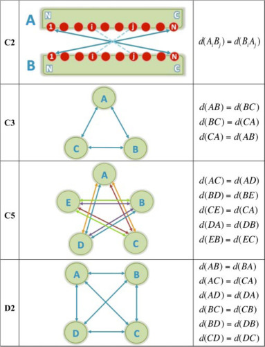
To make use of CN symmetry parameters, one should first activate the use of such restraints using the sym_on = true parameter!
Parameters used to define segments on which symmetry must be enforced are always composed of 6 information (divided into three sections, separated by underscores _), that must be provided:
- The prefix section:
- Symmetry type: the parameter must start with
cNsym_as a prefix, whereNis an integer defining the symmetry type (e.g.:c2sym_), allowing haddock3 to understand how many partners should be expected and how to automatically build the symmetry distance restraints.
- Symmetry type: the parameter must start with
- The infix section:
- Starting residue: using the infix
sta(for start), defines the first residue in the CN symmetry segment. - Ending residue: using the infix
end(for end), defines the last residue in the CN symmetry segment. - ChainID/SegmentID: using the infix
seg(for segment), defines the segmentID in the CN symmetry segment. - Partner index: after the infix, must be set an integer defining the partner (e.g.:
seg1). This index is used to group parameters related to the same partner together and match the start, end, and segment ID.
- Starting residue: using the infix
- The suffix section:
- Symmetry index: the suffix (
_Y) must be define the index of the symmetry. This allows the definition of multiple CN symmetries at the same time.
- Symmetry index: the suffix (
Note that multiple symmetry restraints can be set up in the same run.
This is performed by adding the index (_Y) to the parameter name (e.g: cNsym_xxx_Y)
The first definition must always start with an index of 1 (_1)!
Here is an example of how to define two C3 symmetries:
# Activation of the symmetry restraints
sym_on = true  # Very important, otherwise nothing will be considered
# Tune the force constant
ksym = 10.0  # Here default parameter is shown for the purpose of this manual

###################################
# First definition of C3 Symmetry #
###################################
## PRFIX:  c3sym_ is used to define C3 symmetry
## INFIX:  `sta`, `end`, `seg` must be defined for the 3 segments
## SUFFIX: _1 is used (as it's the first definition of C3 symmetry)
####################################
# Definition of the first partner
c3sym_sta1_1 = 1    # Residue number of the first residue in the first C3 symmetry segment
c3sym_end1_1 = 30   # Residue number of the last residue in the first C3 symmetry segment
c3sym_seg1_1 = "A"  # Segment ID (chain ID) of this segment
# Definition of the second partner
c3sym_sta2_1 = 1    # Residue number of the first residue in the first C3 symmetry segment
c3sym_end2_1 = 30   # Residue number of the last residue in the first C3 symmetry segment
c3sym_seg2_1 = "B"  # Segment ID (chain ID) of this segment
# Definition of the third partner
c3sym_sta3_1 = 1    # Residue number of the first residue in the first C3 symmetry segment
c3sym_end3_1 = 30   # Residue number of the last residue in the first C3 symmetry segment
c3sym_seg3_1 = "C"  # Segment ID (chain ID) of this segment

####################################
# Second definition of C3 Symmetry #
####################################
## PRFIX:  c3sym is used to define C3 symmetry
## INFIX:  `sta`, `end`, `seg` must be defined for the 3 segments
## SUFFIX: _2 is used (as it's the second definition of C3 symmetry)
####################################
# Definition of the first partner
c3sym_sta1_2 = 31
c3sym_end1_2 = 60
c3sym_seg1_2 = "A"
# Definition of the second partner
c3sym_sta2_2 = 31
c3sym_end2_2 = 60
c3sym_seg2_2 = "B"
# Definition of the third partner
c3sym_sta3_2 = 31
c3sym_end3_2 = 60
c3sym_seg3_2 = "C"
It is also possible to tune the force constant for the CN symmetries using the ksym parameter.
We are providing an example of protein-homotrimer docking using haddock3 here.
S3 symmetry
To make use of S3 symmetry parameters, one should first activate the use of such restraints using the sym_on = true parameter!
It is also possible to tune the force constant for the S3 symmetry using the ksym parameter.
DNA & RNA restraints
Often, you will want to keep DNA / RNA base-pairing fixed during a simulation. Without any restraints, the pairing can fall apart when running semi-flexible refinements or molecular dynamics simulations.
A dedicated parameter can be turned on to automatically discover base pairs and generate restraints between nucleotides to keep them together.
For this, simply set the dnarest_on to true (dnarest_on = true) in the corresponding CNS modules (mainly [flexref] and [mdref]).
Note that while the parameter name only contains DNA in its name, it is also functional for RNA!
Contact restraints
Contact restraints can be automatically defined and set up in CNS modules (mainly [flexref] and [mdref]).
Contact restraints can be automatically defined and set up in CNS modules (mainly [flexref] and [mdref]).
By turning on the contactairs parameter (contactairs = true), HADDOCK will first search for current contacts in the input complex and define restraints to make sure to retain the contact during the simulation step.
This can be useful when complexes where obtained using Center of Mass restraints (cmrest = true) at the [rigidbody] stage, or in refinement scenarios.
By turning on the contactairs parameter (contactairs = true), HADDOCK will first search for current contacts in the input complex and define restraints to make sure to retain the contact during the simulation step.
This can be useful when complexes where obtained using Center of Mass restraints (cmrest = true) at the [rigidbody] stage.
Custom symmetry restraints
If the type of symmetries already implemented in haddock3 is not sufficient for your needs, you can always supply your own symmetry restraint file.
This is performed by defining the path to this file using the symtbl_fname = custom_symmetry_restraints.tbl parameter.
This parameter is available in [rigidbody], [flexref], [emref] and [mdref] modules.
For more details on how to define symmetry restraints, please refer to the Xplor documentation, Distance Symmetry Restraints.
Automated restraints generation
Symmetry restraints
CNS modules using restraints, such as [rigidbody], [flexref], [emref] or [mdref], are also capable of handling symmetry restraints.
This can be very useful when you know that the system you are working with contains such property, and you wish to enforce sampled solutions to be symmetrical.
Various symmetry restraints are already available in Haddock3. But custom symmetry restraints can also be provided. To learn more about them, read the custom symmetry section.
Pre-defined symmetry restraints
3 types of symmetry restraints have been implemented in haddock3:
- Non-crystallographic symmetry: Restraining the conformation to be identical
- Rotational symmetries: where C2, C3, C4, C5 and C6 symmetry can be enforced between selected partners.
- S3 symmetry: The S3 rotational and translational symmetry.
They are described in more detail below.
Here is a related research article describing some of the available symmetries in HADDOCK: E. Karaca, A.S.J. Melquiond, S.J. de Vries, P.L. Kastritis and A.M.J.J. Bonvin Building macromolecular assemblies by information-driven docking: Introducing the HADDOCK multi-body docking server. Mol. Cell. Proteomics, 9, 1784-1794 (2010). Download the final author version here.
Non-crystallographic symmetry
Non-crystallographic symmetry (NCS) restraints are a type of restraints available in CNS. While symmetry is in the name, there is in fact no symmetry involved. They simply enforce an RMSD = 0 between the selected segments, independently of any rotation and/or translation, restraining the conformations to be similar.
To make use of NCS parameters, one should first activate the use of such restraints using the ncs_on = true parameter!
NCS restraints are defined between two partners, but multiple NCS restraints can be set up in the same run.
Parameters used to define NCS restraints are always composed of 6 information (divided into three sections, separated by underscores _), that must be provided:
- The prefix section:
- Symmetry type: the parameter must start with
ncs_as a prefix, indicating haddock3 on what type of symmetry restraints we are dealing with.
- Symmetry type: the parameter must start with
- The infix section:
- Starting residue: using the infix
sta(for start), defines the first residue in the NCS restraint segment. - Ending residue: using the infix
end(for end), defines the last residue in the NCS restraint segment. - ChainID/SegmentID: using the infix
seg(for segment), defines the segment ID in the CNS restraint segment. - Partner index: after the infix, must be set an integer defining the partner (e.g.:
seg1). This index is used to group parameters related to the same partner together and match the start, end, and segment ID.
- Starting residue: using the infix
- The suffix section:
- Symmetry index: the suffix (
_Y) must start for one and define the index of the symmetry. This allows the definition of multiple CN symmetries at the same time and properly attribute the parameters.
- Symmetry index: the suffix (
It is also possible to tune the force constant for the NCS symmetries restraints using the kncs parameter.
Here is an example on how to define a NCS restraints:
# Activation of the NCS restraints
ncs_on = true  # Very important, otherwise nothing will be considered
# Tune the force constant
kncs = 1.0  # Here default parameter is shown for the purpose of this manual

################################
# Definition of NCS restraints #
################################
## PRFIX:  ncs_ is used to define NCS restraints
## INFIX:  `sta`, `end`, `seg` must be defined for the 3 segments
## SUFFIX: _1 is used (as it's the first definition of C3 symmetry)
####################################
# Definition of the first partner
ncs_sta1_1 = 1    # Residue number of the first residue in the first C3 symmetry segment
ncs_end1_1 = 30   # Residue number of the last residue in the first C3 symmetry segment
ncs_seg1_1 = "A"  # Segment ID (chain ID) of this segment
# Definition of the second partner
ncs_sta2_1 = 1    # Residue number of the first residue in the first C3 symmetry segment
ncs_end2_1 = 30   # Residue number of the last residue in the first C3 symmetry segment
ncs_seg2_1 = "B"  # Segment ID (chain ID) of this segment
Note that for the use of NCS restraints:
- starting and ending residues MUST be the same.
- chains/segments must be different.
- the two partners must have the same sequence and residue numbering.
We have dedicated functions to assess the validity of the NCS parameters.
Rotational symmetry
Rotational symmetries (C symmetries) can be enforced between partners. Currently, C2, C3, C4, C5 and C6 symmetries are available. Each symmetry type (CN) must be defined between N partners to be valid.
To make use of CN symmetry parameters, one should first activate the use of such restraints using the sym_on = true parameter!
Parameters used to define segments on which symmetry must be enforced are always composed of 6 information (divided into three sections, separated by underscores _), that must be provided:
- The prefix section:
- Symmetry type: the parameter must start with
cNsym_as a prefix, whereNis an integer defining the symmetry type (e.g.:c2sym_), allowing haddock3 to understand how many partners should be expected and how to automatically build the symmetry distance restraints.
- Symmetry type: the parameter must start with
- The infix section:
- Starting residue: using the infix
sta(for start), defines the first residue in the CN symmetry segment. - Ending residue: using the infix
end(for end), defines the last residue in the CN symmetry segment. - ChainID/SegmentID: using the infix
seg(for segment), defines the segmentID in the CN symmetry segment. - Partner index: after the infix, must be set an integer defining the partner (e.g.:
seg1). This index is used to group parameters related to the same partner together and match the start, end, and segment ID.
- Starting residue: using the infix
- The suffix section:
- Symmetry index: the suffix (
_Y) must be define the index of the symmetry. This allows the definition of multiple CN symmetries at the same time.
- Symmetry index: the suffix (
Note that multiple symmetry restraints can be set up in the same run.
This is performed by adding the index (_Y) to the parameter name (e.g: cNsym_xxx_Y)
The first definition must always start with an index of 1 (_1)!
Here is an example of how to define two C3 symmetries:
# Activation of the symmetry restraints
sym_on = true  # Very important, otherwise nothing will be considered
# Tune the force constant
ksym = 10.0  # Here default parameter is shown for the purpose of this manual

###################################
# First definition of C3 Symmetry #
###################################
## PRFIX:  c3sym_ is used to define C3 symmetry
## INFIX:  `sta`, `end`, `seg` must be defined for the 3 segments
## SUFFIX: _1 is used (as it's the first definition of C3 symmetry)
####################################
# Definition of the first partner
c3sym_sta1_1 = 1    # Residue number of the first residue in the first C3 symmetry segment
c3sym_end1_1 = 30   # Residue number of the last residue in the first C3 symmetry segment
c3sym_seg1_1 = "A"  # Segment ID (chain ID) of this segment
# Definition of the second partner
c3sym_sta2_1 = 1    # Residue number of the first residue in the first C3 symmetry segment
c3sym_end2_1 = 30   # Residue number of the last residue in the first C3 symmetry segment
c3sym_seg2_1 = "B"  # Segment ID (chain ID) of this segment
# Definition of the third partner
c3sym_sta3_1 = 1    # Residue number of the first residue in the first C3 symmetry segment
c3sym_end3_1 = 30   # Residue number of the last residue in the first C3 symmetry segment
c3sym_seg3_1 = "C"  # Segment ID (chain ID) of this segment

####################################
# Second definition of C3 Symmetry #
####################################
## PRFIX:  c3sym is used to define C3 symmetry
## INFIX:  `sta`, `end`, `seg` must be defined for the 3 segments
## SUFFIX: _2 is used (as it's the second definition of C3 symmetry)
####################################
# Definition of the first partner
c3sym_sta1_2 = 31
c3sym_end1_2 = 60
c3sym_seg1_2 = "A"
# Definition of the second partner
c3sym_sta2_2 = 31
c3sym_end2_2 = 60
c3sym_seg2_2 = "B"
# Definition of the third partner
c3sym_sta3_2 = 31
c3sym_end3_2 = 60
c3sym_seg3_2 = "C"
It is also possible to tune the force constant for the CN symmetries using the ksym parameter.
We are providing an example of protein-homotrimer docking using haddock3 here.
S3 symmetry
To make use of S3 symmetry parameters, one should first activate the use of such restraints using the sym_on = true parameter!
It is also possible to tune the force constant for the S3 symmetry using the ksym parameter.
DNA & RNA restraints
Often, you will want to keep DNA / RNA base-pairing fixed during a simulation. Without any restraints, the pairing can fall apart when running semi-flexible refinements or molecular dynamics simulations.
A dedicated parameter can be turned on to automatically discover base pairs and generate restraints between nucleotides to keep them together.
For this, simply set the dnarest_on to true (dnarest_on = true) in the corresponding CNS modules (mainly [flexref] and [mdref]).
Note that while the parameter name only contains DNA in its name, it is also functional for RNA!
Contact restraints
Contact restraints can be automatically defined and set up in CNS modules (mainly [flexref] and [mdref]).
Contact restraints can be automatically defined and set up in CNS modules (mainly [flexref] and [mdref]).
By turning on the contactairs parameter (contactairs = true), HADDOCK will first search for current contacts in the input complex and define restraints to make sure to retain the contact during the simulation step.
This can be useful when complexes where obtained using Center of Mass restraints (cmrest = true) at the [rigidbody] stage, or in refinement scenarios.
By turning on the contactairs parameter (contactairs = true), HADDOCK will first search for current contacts in the input complex and define restraints to make sure to retain the contact during the simulation step.
This can be useful when complexes where obtained using Center of Mass restraints (cmrest = true) at the [rigidbody] stage.
Custom symmetry restraints
If the type of symmetries already implemented in haddock3 is not sufficient for your needs, you can always supply your own symmetry restraint file.
This is performed by defining the path to this file using the symtbl_fname = custom_symmetry_restraints.tbl parameter.
This parameter is available in [rigidbody], [flexref], [emref] and [mdref] modules.
For more details on how to define symmetry restraints, please refer to the Xplor documentation, Distance Symmetry Restraints.
Ab-initio / naive docking protocols
While HADDOCK is meant to use information from experiments, literature, or bioinformatic predictions to guide the sampling during the docking, sometimes such data is not available. For these reasons, dedicated parameters can be turned on to perform ab-initio docking.
Three different ways of doing ab-initio docking in haddock3 are discussed below.
Prior considerations
- Ab-initio docking typically involves limited, if any, prior information on how the various chains involved should interact. As a result, producing good solutions relies heavily on a trial-and-error approach. Thus, to enhance the likelihood of generating good models, we strongly advise increasing the sampling at the
[rigidbody]docking stage (by tuning thesamplingparameter). - The next three ab-initio docking solutions described below are incompatible with each other, and you should not turn on multiple of them at the same time.
Center of mass restraints
Turning on the center of mass restraints parameter (cmrest = true), will automatically generate restraints between the centers of masses of the different chains present in the system, and use these restraints during the docking.
This parameter goes together with the cmtight parameter, which controls how the upper limit distance is defined for the center of mass restraints.
To calculate the upper distance limit for the restraints, the height, width, and depth of each molecule are first determined. Technically, each molecule is aligned along its principal (i.e. longest) components, and the x, y, and z dimensions are measured. Next:
- If
cmtight=true: The 'molecule distance' for each molecule is calculated as the average of the two smallest dimensions, each divided by 2. For example:
- If
cmtight=false: The 'molecule distance' is the average of all three half-dimensions:
- For DNA, RNA, small ligands, or glycans: The 'molecule distance' is set to 0.
The effective upper distance limit for the center of mass distance restraint is defined as the sum of the molecule distances of all molecules involved.
Lastly, the strength of the center of mass restraints can be controlled via the force constant (kcm)
cmrest, cmtight and kcm parameters are accessible in [rigidbody], [flexref] and [mdref] modules.
Please note that setting cmrest = true is suitable for globular structures, but may deform other types of molecules, e.g. fibrous proteins, long bDNA etc., as restraint will be defined to the center of the molecule.
Random Ambiguous Restraints
Another solution for ab-initio docking is to generate random ambiguous restraints (AIRs).
This is performed by turning on the ranair parameter (ranair = true) in the [rigidbody] module.
When ranair is turned on:
- During the rigid-body sampling, residues on the surface of each chain are randomly selected, along with surrounding ones, to define a patch.
- Ambiguous restraints are then generated between these patches, and rigid-body minimization is performed.
ranair parameter is limited to the docking of two chains only, and no other type of restraints will be considered, even if specified in the configuration file.
Note that during the later stages of the docking workflow (e.g., [flexref], [emref], [mdref]), it is advisable to enable the contactairs = true parameter to ensure the molecules remain held together at the interface. This setting defines restraints between thwe residues within a 5Å distance between molecules. However, be aware this may generate a large number of restraints, potentially slowing down computations.
Surface restraints
An alternative solution for ab-initio docking is to turn on the surfrest parameter (surfrest = true).
By doing so, surface residues are identified, and contact restraints between these residues across docking partners are generated on the fly.
These restraints are defined as ambiguous distance restraints between all backbone atoms (CA, BB, or N1) of the two molecules. For small ligands, all atoms are considered.
If fewer than 3 CA and P atoms are found, all atoms are selected instead.
The upper distance limit is set to 7Å for standard molecules and 4.5Å for small ligands.
Such restraints can be particularly useful in multi-body (N>2) docking to ensure that all molecules are in contact and thus promote compactness of the docking solutions. Similarly to the random AIRs, surface contact restraints can be used in ab-initio docking. In such a case it is important to have sufficient sampling of the random starting orientations, which significantly increases the number of structures generated by the rigid-body docking.
Note that this option is computationally more expensive than center of mass restraints and random AIRs, as the number of restraints grows exponentially with the number of residues in the system.
Also, because of the high number of restraints, the physico-chemical components of the scoring function can be masked by the noise of the AIRs component.
Therefore setting the weight of the AIR component to 0 (w_air = 0) could help the scoring function to better decipher between model conformations.
This parameter goes along with its force constant ksurf, which can be tuned to control the strength of the surface restraints.
Flexibility options in Haddock3
In the refinement modules of Haddock3, a molecule or parts of it (i.e., its segment(s)) can be treated as:
- Rigid: The entire chain is treated as rigid throughout all phases of the module's protocol.
- Semi-flexible: One or several segments of the chain are treated as rigid during the initial phases of the protocol and as fully flexible during the final phases.
- Fully flexible: One or more segments of the chain are treated as fully flexible during all phases of the protocol.
By default, semi-flexible and rigid segments of docking partners are determined automatically based on interface contacts. Automatically defined semi-flexible segments include residues within the interface, meaning residues that are 5Å or closer to residues in another molecule. The remaining segments comprising residues outside of the interface are automatically defined as rigid. By default, no segments are defined as fully flexible.
Flexibility can be defined in any of the CNS model refinement modules, namely: [emref], [flexref], and [mdref].
Check out schematic images of the refinement protocols employed in different refinements modules:
Below you can find explanations and examples on the definition of different types of segments:
Automatic Definition of Rigid and Semi-Flexible Segments
As this behaviour is enabled by default, there is no need to add any parameters to the tolm file.
Internally, this behaviour is controlled by the nsegX parameter, which specifies the number of semi-flexible segments for molecule X. Here, X corresponds to the sequential number of the molecule in the input, i.e. the order in which input PDB files are given.
For example:
- If no manual flexibility is defined and two docking partners are provided, Haddock3 will proceed with:
nseg1 = -1; nseg2 = -1 - For three docking partners, the parameters will be:
nseg1 = -1; nseg2 = -1; nseg3 = -1
And so on, for additional molecules.
The default value of -1 indicates that the semi-flexible and rigid segments are automatically defined based on the molecule's interface residues.
Manual definition
Rigid Molecule
To keep an entire molecule rigid throughout the refinement, the nsegX parameter for that molecule should be set to 0.
Example: Keeping the Protein Molecule Rigid
Consider a docking protocol involving two molecules: DNA and protein, where DNA is the 1st molecule and protein is the 2nd by the order of the input. This order is important!
To treat the protein as a rigid body during flexible refinement, set the parameter nseg2 to 0. The corresponding .cfg file would look as follows:
# Input molecules: DNA as the 1st molecule, and protein as the 2nd
molecules = ["DNA.pdb", "protein.pdb"]

# ...

[flexref]
# Keep the protein rigid
nseg2 = 0

# No definition for nseg1, so it is set to -1 by default.
# This means the DNA molecule will have its rigid and semi-flexible segments
# automatically defined based on interface residues.
Semi-flexible Segment
To manually define a semi-flexible segment, the user must specify the first and last residues of the segment using the parameters seg_sta_X_Y and seg_end_X_Y, respectively.
Parameter Details:
Xis the sequential number of the molecule (i.e. position of the PDB file in the input) to which the segment belongs. This follows the same logic asXinnsegXparameter, explained above.Yis the sequential number of the segment being defined. This allows multiple semi-flexible segments to be defined within the same molecule.- The values of
seg_sta_X_Yandseg_end_X_Ymust be integers and must correspond to residue indices present in the corresponding input PDB file.
Example: Two Semi-Flexible Segments of DNA
Consider a docking scenario with two partners: a DNA molecule and a protein, where two segments of the DNA are manually defined as semi-flexible.
- The first segment includes residues 2 to 19.
- The second segment includes residues 22 to 39.
The DNA molecule is defined as the 1st partner, and the protein as the 2nd. This order is important!
To define the semi-flexible segments:
- The first segment (suffix _1) starts at residue 2 and ends at residue 19.
- The second segment (suffix _2) starts at residue 22 and ends at residue 39. The corresponding .cfg file would look as follows:
# Input molecules: DNA as the 1st molecule, and protein as the 2nd
molecules = ["DNA.pdb", "protein.pdb"]

# ...

[flexref]
# Define the first segment (suffix _1) for DNA (X = 1) between residues 2 and 19
seg_sta_1_1 = 2
seg_end_1_1 = 19

# Define the second segment (suffix _2) for DNA (X = 1) between residues 22 and 39
seg_sta_1_2 = 22
seg_end_1_2 = 39
Fully flexible Segment
Fully Flexible Segment
The manual definition of a fully flexible segment differs slightly from the definition of a semi-flexible segment. For fully flexible segments, the user must specify the first and last residues of the fully flexible segment using the parameters fle_sta_Y and fle_end_Y. On top of it, the user must define the chain ID (instead of the molecule's sequential number) using the parameter fle_seg_Y.
Parameter Details:
Ydefines the sequential number of the segment being defined. This allows multiple semi-flexible segments to be defined within the same chain.- The value of
fle_seg_Yis a string and must correspond to the chainID/segemntID present in one of the input PDB files. - The values of
seg_sta_X_Yandseg_end_X_Ymust be integers and must correspond to residue indices present in chain/segment defined by `fle_seg_Y.
Example: Fully Flexible Glycan
Let's consider a docking scenario involving two partners, namely a protein (chain A) and a glycan (chain B, consisting of 4 residues, numbered strating from 1), where the entire chain of glycan is manually defined as fully flexible.
Let's define the protein as the 1st docking partner and the glycan as the 2nd docking partner in .cfg file.
Then, to define glycan as fully flexible, its entire chain should be treated a single segment, i.e.:
- the chainID is set to 'B'
- the starting residue is set to 1
- the ending residue is set to 4
The corresponding .cfg file would look as follows:
molecules = [
 "protein.pdb", # chain A
 "glycan.pdb"   # chain B, residues from 1 to 4
 ]

# ...

[flexref]
# Define chain ID of 1st fully flexible segment
fle_seg_1 = "B"
# Define the first residue for the 1st fully flexible segment
fle_sta_1 = 1
# Define the last residue for the 1st fully flexible segment
fle_end_1 = 4
Workflow configuration file
Haddock3 uses a configuration file to define the workflow to be performed. A workflow is defined in simple configuration text files, similar to the TOML format but with extra features.
It basically contains two main parts:
- Global parameters: General parameters to be applied to the workflow, including input molecules and location where to run the docking protocol.
- List of modules: Sequence of [module names], defining the sequential order in which each module must be performed. Each module has several parameters, that can be defined to fine-tune them, or left untouched therefore using default parameters.
Examples of workflow configuration files are available here !
Schematic representation of a haddock3 workflow configuration file
Let's consider the definition of a Haddock3 configuration file named schematic_workflow.cfg:
###############################################
# First, we will define the GLOBAL PARAMETERS #
###############################################
### MANDATORY PARAMETERS
# The run directory
run_dir = "super_example"
# The input molecules
molecules = ["antibody.pdb", "antigen.pdb"]
### EXECUTION PARAMETERS
# Running in 'local' mode (also default)
mode = "local"
# Setting the number of cores to 10
ncores = 10
### POST PROCESSING AND CLEANING PARAMETERS
postprocess = true  # will run `haddock3-analyse` and generate graphs
clean = true  # Will compress output pdb files

#############################################################
# Now, we define the list of [modules] and their parameters #
#############################################################
# Using moduleX as first module in the workflow
[moduleX]
param1 = "super_string"
param2 = 2
param3 = [2, 3, 4]

# Using moduleY as second module in the workflow
[moduleY]
param1 = 5.5
param2 = "fine_tune"

# Re-using moduleX as last module in the workflow with different parameters
[moduleX]
param1 = "other_string"
param4 = 3.33
note that this configuration file is only schematic and not functional as modules [moduleX] and [moduleY] do not exist in haddock3.
This configuration file can then be executed by running:
haddock3 schematic_workflow.cfg
Click here for more details about the haddock3 command line interface.
Global parameters
Global parameters must be defined before any use of [modules], as they will act on every downstream [modules].
Three types of global parameters are defined:
- Mandatory: These global parameters must be defined for a configuration file to be valid and properly executed.
- Execution: The execution parameters are related to the execution mode of haddock3, enabling to either run with local cores, use schedulers (such as slurm or torque) or even spread the workload over multiple nodes using MPI.
- Optional: These optional parameters are mostly related to pre- and post-processing of the results.
Mandatory global parameters
Two mandatory parameters are required to perform a haddock3 run:
run_dir: Define the directory path where the run will take place (e.g:run_dir = "docking_run")molecules: A coma-separated list of paths to input molecules. Note that each input file can be a conformational ensemble of the same molecule. Currently limited to a maximum number of 20 input files. (e.g.:molecules = ["receptor.pdb", "protein.pdb"])
Execution global parameters
Various parameters are related to the execution modes:
ncores: Maximum number of cores to be used by the haddock3 run. If set to a higher number of cores than the ones available on the system, it will be tuned down and limited to use all available cores.max_cpus: When set totrue, uses all cores set by thencoresparameter. Iffalse, remove 1 core fromncores, ensuring the computer to still be able to perform tasks outside of haddock3. The default istrue.- The
modeparameter allows to define the execution mode of haddock3.- Using 'local', allows to run haddock3 using the local resources, bound to the operating system
- In 'batch' mode, haddock3 will send jobs to the queue of your choice (defined by the
batch_typeandqueueparameters). Note that when using the 'batch' mode, you should also define parameters such as (batch_type,queue,queue_limit,concat) - In 'mpi' mode, haddock3 will spread the workload over the available nodes.
batch_type: defines which batch submission tool must be used, between 'slurm' and 'torque'. Note that this requires your computing engine to have access to such kind of queuing system.queue: name of the queue on which the submission should be performed. This allows to target queues that can process shorter / longer jobs. It requires you to have an estimation of how long your job will last.queue_limit: Sets the number of jobs to submit to the batch system. The default is 100.concat: Number of models to produce per job to send to the batch system. If set to a value above 1, multiple models can be calculated within one job. The default is 1.self_contained: When set totrue, this option will copy the CNS scripts and executable to the run folder, making it a self-contained run. The default isfalse.clean: When set totrue, clean the modules directory if the run succeeds by compressing or removing output files. The default istrue.offline: When set totrue, completely isolate the haddock3 run and results from internet. This option is useful when no internet connection is available. Default isfalse.debug: By setting it tofalse, reduces the amount of I/O operations, often speeding up the process. When set totrue, input files, intermediate files and output files are generated and kept, which is useful when tracking potential errors. The default isfalse.
Local mode
Often the prefered execution mode if you submit a haddock3 run to a queuing system or run on your own computer.
The local mode (targeted using the global parameter mode = 'local'), utilize the operating system device to perform the computations.
Setting the ncores parameter allows to tune the number of CPU cores to use during the run.
Note that if you set this value too high compared to your system capabilities, this value will be automatically scaled down to the maximum number of cores available on the machine.
Batch mode
Utilise queuing system machinery to submit CNS runs.
batch_type: defines which batch submission tool must be used, between 'slurm' and 'torque'. Note that this require your computing engine to have access to such kind of queuing system.queue: name of the queue on which the submission should be performed. This allows to target queues that can process shorter / longer jobs. It requires you to have an estimation of how long your job will last.queue_limit: Sets the number of jobs to submit to the batch system. Default is 100.concat: Number of models to produce per job to send to the batch system. If set to a value above 1, multiple models can be calculated within one job. The default is 1.
MPI mode
Requires the installation of the mpi4py python library and OpenMPI to be installed on the operating system.
Optional global parameters
postprocess: When set totrue, executeshaddock3-analyseon the CAPRI folders at the end of the run. The default istrue.preprocess: When set totrue, tries to correct input PDBs before the workflow. The default isfalse.gen_archive: By setting it totrue, at the end of the workflow, the entirerun_dirwill be compressed as a.tgzarchive. In addition, theanalysisdirectory will be archived too, and a local copy of models will be made in it. This allows to reduce the number of files to be transferred and make the analysis directory self-sufficient. Useful for the web application and if only the last models generated by the workflow are required. The default isfalse.
Modules in haddock3
Haddock3 has this particularity (compared to the pervious HADDOCK2.X versions), that there is not a single static workflow to be processed, but rather a custom one requiring the user to design their own workflows by placing [modules] one after the other, enabling to generate a sequence of events to solve their research question.
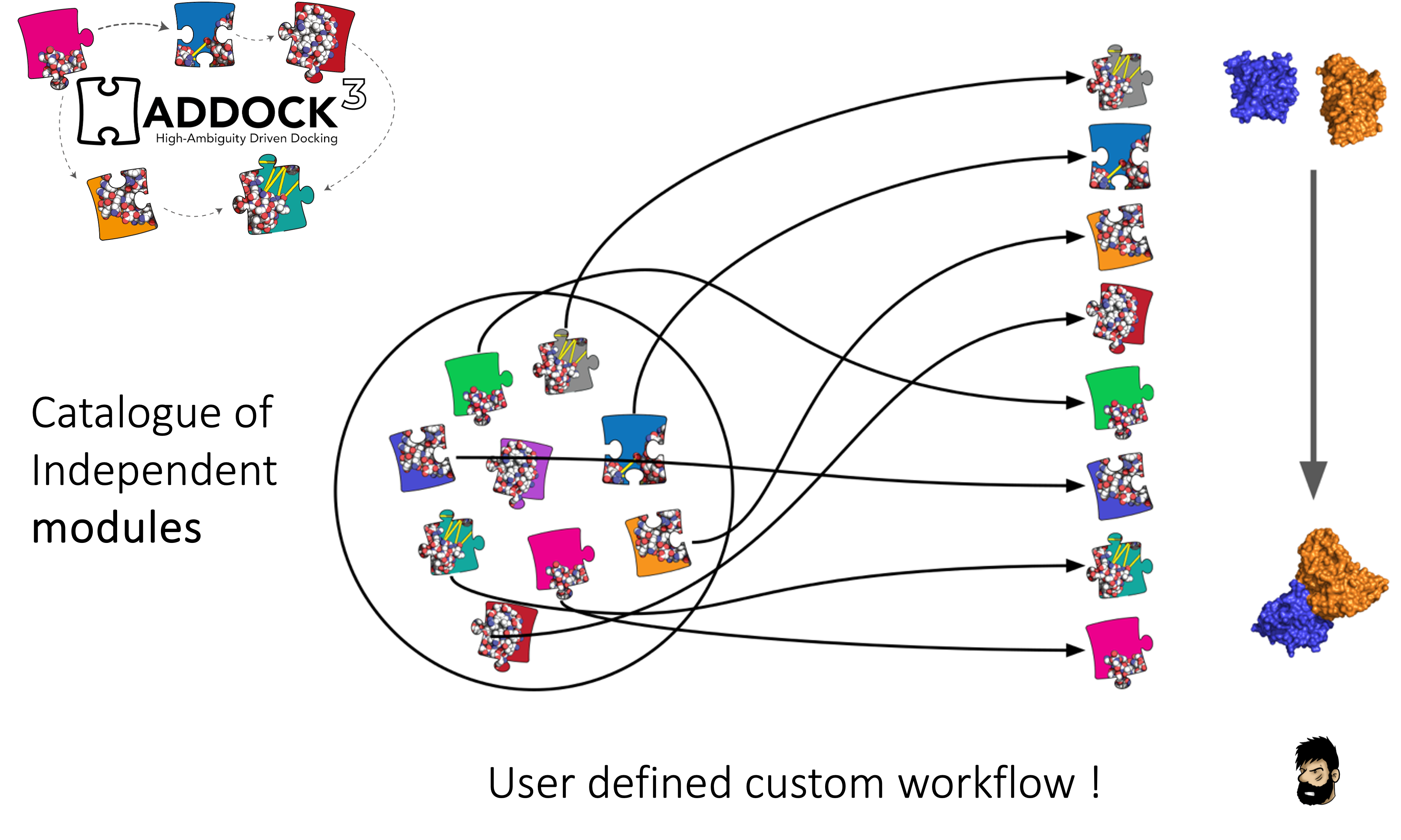
Various [modules] are available in Haddock3, and they are grouped together by types:
- Topology modules: these modules focus in the building of missing atoms and the generation of appropriate topology files enabling downstream use of molecular dynamics protocols.
- Sampling modules: dedicated to performing sampling of initial conformations, such as rigidbody docking.
- Refinement modules: these modules aim at refining interaction interface, using simulated annealing protocol, energy minimization or molecular dynamics with an explicit solvent shell.
- Scoring modules: these modules are evaluating provided complexes with dedicated scoring functions, such as the HADDOCK score.
- Analysis modules: these modules focus on the analysis of docking models. It ranges from the clustering of docking models to the selection of best-ranked ones passing by the evaluation of the models with respect to a reference structure using CAPRI criteria.
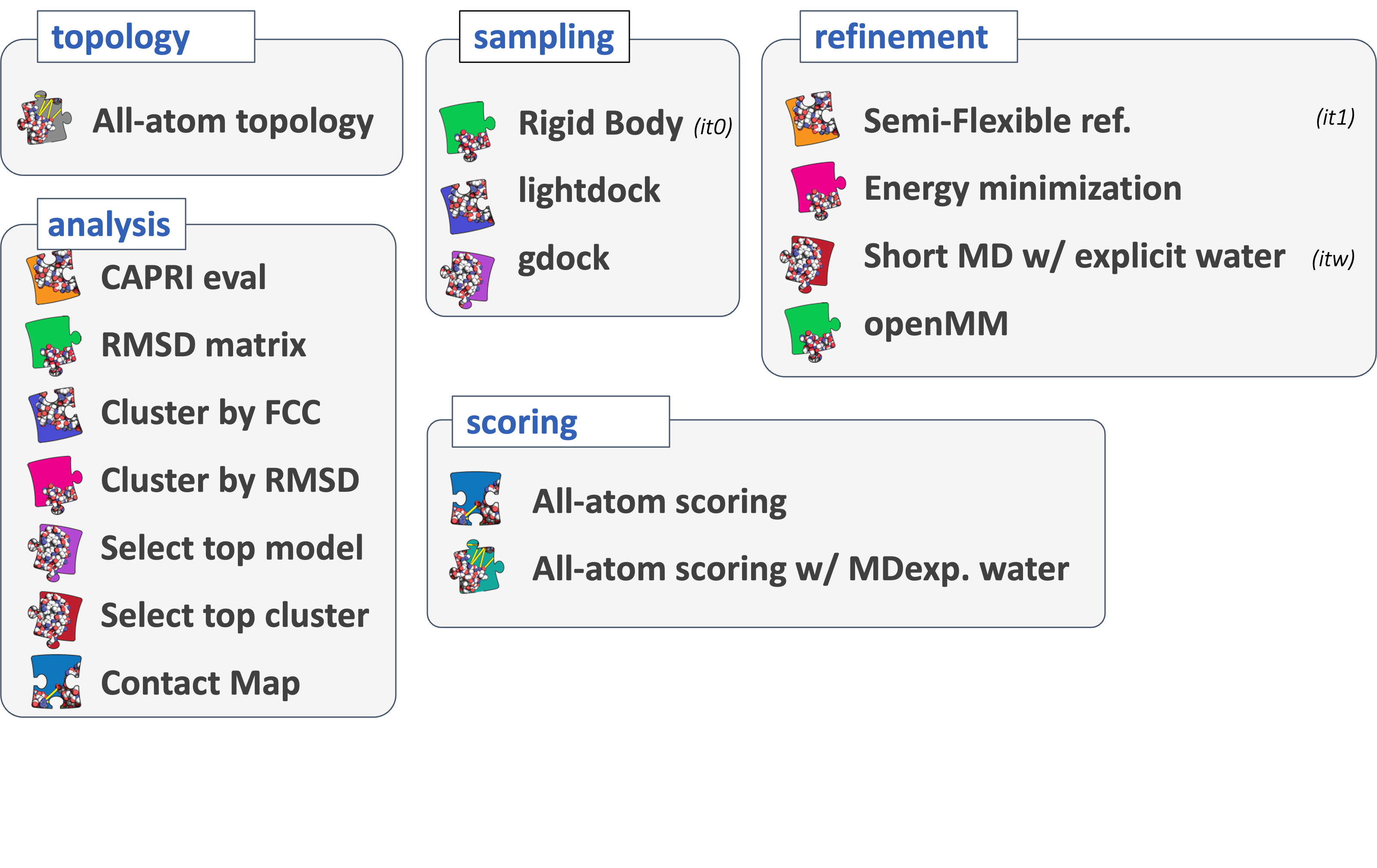
Defining module parameters
To tune module parameters, you first need to define which [module] you will be using, then add the list of parameters and their new values.
Note that if a parameter is not defined, its default value will be used instead.
Tuning a module parameter
In the configuration file, right after declaring which module you want to use, add the parameters and their new values in the subsequent lines.
Here is a synthetic example:
[module]
parameter1 = new_value_1
parameter3 = new_value_3
Note that you can only define one parameter per line.
Definition of default parameter values
Each module has its own default parameter names and values, set in a file named defaults.yaml.
This is used to set default parameters when they are not specified in the configuration file.
The defaults.yaml file is not only used to check if the parameter name exists at execution time, but also as reference to know if the configuration file provided by the use respects the allowed value for a given parameter.
Note for advanced users: If you feel that the parameter range is not suited for your research, you can always tune the defaults values or the maximum values that can be adopted by this parameter, by editing the defaults.yaml file inside the module directory (at your own risk).
Set of available modules
Below is presented the list of available modules.
For detailed explanation of each module and their respective parameters, please refer to the online documentation.
You can also use the haddock3-cfg command line to get information on each module and their parameters (documentation here).
Topology modules
[topoaa]: Builds missing atoms and generates the all-atom topologies for the CNS engine.[topocg]: coming soon
Sampling modules
[rigidbody]: Rigid body energy minimization with CNS (previously known asit0in HADDOCK2.X series).[gdock]: Third-party genetic algorithm-based docking software.[lightdock]: Third-party Glow-worm Swarm Optimisation (GSO) docking software.
Refinement modules
[flexref]: Semi-flexible refinement using a simulated annealing protocol through molecular dynamics simulations in torsion angle space (previously known asit1in HADDOCK2.X series).[emref]: Refinement by energy minimization (previously known asitw EM onlyin HADDOCK2.4).[mdref]: Refinement by a short molecular dynamics simulation in explicit solvent (previously known asitwin HADDOCK2.X series).[openmm]: Short molecular dynamics simulation (in explicit or implicit solvent) using the OpenMM library.
Scoring modules
- CNS scoring modules:
[emscoring]: Scoring of a complex performing a short EM (builds the topology and all missing atoms).[mdscoring]: Scoring of a complex performing a short MD in explicit solvent + EM (builds the topology and all missing atoms).
[prodigyprotein]: Binding affinity prediction of a protein-protein complex by theprodigytool.[prodigyligand]: Binding affinity prediction of a protein-ligand complex by theprodigy-ligandtool.
Analysis modules
- Analysis:
[alascan]: Performs alanine (or other residue) scanning on the models generated in the previous step.[caprieval]: Calculates CAPRI metrics (i-RMDS, l-RMSD, Fnat, DockQ, RMSD) with respect to the top scoring model or reference structure if provided.[contactmap]: Calculates the contact maps for the models generated in the previous step.
- Clustering:
[rmsdmatrix]: Calculates the pairwise RMSD matrix between all the models generated in the previous step.[ilrmsdmatrix]: Calculates the pairwise interface-ligand-RMSD (iLRMSD) matrix between all the models generated in the previous step.[clustrmsd]: Clusters models based on pairwise RMSD matrix previously computed by either the calculated with the[rmsdmatrix]or[ilrmsdmatrix]modules.[clustfcc]: Clusters models based on the fraction of common contacts (FCC)
- Selection:
[seletop]: Select the top N models from the previous step.[seletopclusts]: Selects top N clusters from the previous step.[filter]: Filter models based on their score and a defined threshold value.
Developing a new module
Haddock3 is a collaborative project, and researchers can contribute to it, increasing the scope and potential of the Haddock3 suite. Information on how to contribute and setup a proper development environment is available on the GitHub repository:
- CONTRIBUTING.md, contains information on how to contribute.
- DEVELOPMENT.md, contains information on how to set up an adequate development environment.
Name
Modules
More than 15 modules are currently available in HADDOCK3, grouped by category:
Topology modules
[topoaa] module
The [topoaa] module is dedicated to the generation of CNS compatible parameters (.param) and topologies (.psf) for each of the input structures.
It will:
- Detect missing atoms, including hydrogens
- Re-build them when missing
- Build and write out topologies (
.psf) and coordinates (.pdb) files
This module is a prerequisite to run any downstream modules using CNS.
Having access to parameters and topology is mandatory for any kind of EM/MD related tasks.
Therefore this is the reason why the module [topoaa] is often used as first module in a workflow.
Note that for non-standard bio-molecules (apart from standard amino-acids, some modified ones, DNA, RNA, ions and carbohydrates ... see detailed list of supported molecules), such as small-molecules, parameters and topology must be obtained and provided by the user, as there is currently no built-in solution to generate them on the fly.
More information about [topoaa] parameters can be accessed here or retrieved by running:
haddock3-cfg -m topoaa
Here an example configuration file snapshot of a typical execution of the
[topoaa] module in which a user specifies the protonation state of the histidine
residues:
# Definition of
run_dir = "example"
molecules = [
 "DNA_structure.pdb",
 "1abc.pdb",
]

[topoaa]
autohis = false
# Specify molecule 1 specific parameters
[topoaa.mol1]
5_phosphate = true
# Specify molecule 2 specific parameters
[topoaa.mol2]
nhisd = 1
hisd_1 = 76
nhise = 1
hise_1 = 15
charged_nter = true
charged_cter = false

# Workflow continues with other modules
# ...
The [topoaa.mol1] in square brackets is not as module, but allows to specify topoaa parameters for a given molecule.
In this case (mol1), the parameters will be applied to the first molecule in the list of input molecules ("1abc.pdb").
Notable parameters
autohis: If set tofalse, you will need to specify the protonation states of histidines manually.
Parameters specific to each molecule
[topoaa.molX]: Allows the definition of specifictopoaaparameters for molecule X.nhisd,nhiseallow to define the number ofHISD,HISEin the molecule.hisd_Y,hise_Y, allow to define which residue needs to be modified (e.g:hisd_1 = 3means that we are defining the first HISD residue, and this residue has residue index of 3 in the file).charged_nter,charged_cterallow to define the state of Nter and Cter residues. Note that chain breaks are not evaluated as termini residues.5_phosphate: Allows to define the state of the 5' end of nucleic acids sequences. If set totrue, 5' end will be a phosphate group. Otherwise it will be an OH. (default false). Note that chain breaks are not evaluated as 5' ends.
Sampling modules
[rigidbody] module
The [rigidbody] module does a randomization of orientations and rigid-body minimization.
It corresponds to the classical it0 step in the HADDOCK2.x series.
In this module, the interacting partners are treated as rigid bodies, meaning that all geometrical parameters such as bond lengths, bond angles, and dihedral angles are frozen. The partners are first separated in space and randomly rotated around their respective centers of mass. Afterward, the molecules are brought together by rigid-body energy minimisation with rotations and translation as the only degrees of freedom.
The driving force for this energy minimization is the energy function, which consists of the intermolecular van der Waals and electrostatic energy terms and the restraints defined to guide the docking. The restraints are distance-based and can consist of unambiguous or ambiguous interactions restraints (AIRS). In ab-initio docking mode those restraints can be automatically defined in various ways; e.g. between the center of masses (CM restraints) or between randomly selected patches on the surface (random AIRs).
The definition of those restraints is particularly important as they effectively guide the minimization process. For example, with a stringent set of AIRs or unambiguous distance restraints, the solutions of the minimization will converge much better and the sampling can be limited. In ab-initio mode, however, very diverse solutions will be obtained and the sampling should be increased to make sure to sample enough the possible interaction space.
See animation of the rigidbody protocol:
The default HADDOCK scoring function in the rigid-body module is the following:
For a detailed explanation of the components of the scoring function, please have a look here.
Throughout the years, the weights of the scoring function have been optimized for various systems. For example, when dealing with small molecules or glycans, it is recommended to scale up the van der Waals term from 0.1 to 1:
# ...
[rigidbody]
w_vdw = 1.0
# ...
Please refer to the different docking scenarios for more information about how to tune the scoring function for your specific system.
Notable parameters
The most important parameters for the [rigidbody] module are:
ambig_fname: file containing the ambiguous interaction restraints (AIRs)unambig_fname: file containing the unambiguous interaction restraintsrandremoval: whether or not to activate the random removal of restraints (default: True)cmrest: whether or not to use center of mass restraints (default: False)sampling: number of rigid body models to generate (default: 1000)
More information about [rigidbody] parameters can be accessed here or retrieved by running:
haddock3-cfg -m rigidbody
Here an example configuration file snapshot of a typical execution of the
[rigidbody] module:
# ...
molecules = [
 "1abc.pdb",
 "2xyz.pdb"
]

[topoaa]
[rigidbody]
ambig_fname = "ambig.tbl"
unambig_fname = "unambig.tbl"
sampling = 2000 # higher sampling if information is limited
[caprieval]
# ...
[lightdock] module
[gdock] module
Refinements modules
[emref] module
Energy minimization refinement with CNS.
The [emref] module refines the input structure or a complex by energy minimization using
the conjugate gradient method implemented in CNS.
Coordinates of the energy-minimized structures are saved, and each structure/complex is then evaluated using HADDOCK scoring function.
The default HADDOCK scoring function in the [emref] module is the following:
Notable parameters
The most important parameters for the [emref] module are:
ambig_fname: file containing the ambiguous interaction restraints (AIRs, optional)unambig_fname: file containing the unambiguous interaction restraints (optional)randremoval: whether or not to activate the random removal of restraints (default: True)nemsteps: number of energy minimization steps (default: 200)
More information about the [emref] parameters is available here or retrieved by running:
haddock3-cfg -m emref
[flexref] module
Flexible refinement with CNS.
The [flexref] module (previously known as it1 stage in HADDOCK2.X series),
is a semi-flexible simulated annealing (SA) protocol based on molecular
dynamics (MD) in torsion angle space.
This semi-flexible SA consists of four sequential stages:
- High-temperature rigid body MD
- Rigid body SA
- Semi-flexible SA with flexible side-chains at the interface
- Semi-flexible SA with fully flexible interface (both backbone and side-chains)
By default, only the interface regions are treated as semi-flexible. These regions are automatically defined based on intermolecular contacts. However, the user has the option to manually specify semi-flexible regions, and also define fully flexible regions that remain flexible throughout the entire protocol, starting from the high-temperature rigid-body MD stage.
See animation of the `[flexref]` protocol in action:
Here is a schematic visualization of the [flexref] stages with relevant parameters:

The temperature and number of steps for the various stages can be tuned.
The default HADDOCK scoring function in the [flexref] module is the following:
Notable parameters
The most important parameters for the [flexref] module are:
ambig_fname: file containing the ambiguous interaction restraints (AIRs, optional)unambig_fname: file containing the unambiguous interaction restraints (optional)seg_*_X_Y: for the definition of semi-flexible segments (see flexibility section for more information)fle_*_Y: for the definition of fully flexible segments (see flexibility section for more information)
More information about the [flexref] parameters is available here or retrieved by running:
haddock3-cfg -m flexref
[mdref] module
Explicit solvent MD refinement with CNS.
The [mdref] module (previously known as itw in HADDOCK2.X series), is a small MD simulation in cartesian space using explicit solvent.
A layer of solvent (8Å for water, 12.5Å for DMSO) is generated around surface residues.
The [mdref] protocol consists of four sequential steps:
- Short energy minimization
- Heating: 3 stages of short MD to reach the temperature of 300K (gradually increases the temperature, performing MD at 100K, 200K, and finally 300K)
- MD at 300K
- Cooling: 3 stages of short MD to reach the temperature of 100K (gradually decreases the temperature, performing MD at 300K, 200K, and finally 100K)
See animation of the `[mdref]` protocol in action:

Here is a schematic visualization of the [mdref] stages with relevant parameters:
Using this protocol with default parameters, no spectacular changes are expected;
however, the scoring of the various structures may be improved.
The default HADDOCK scoring function in the [mdref] module is the following:
Notable parameters
The most important parameters for the [mdref] module are:
-
ambig_fname: file containing the ambiguous interaction restraints (AIRs, optional) -
unambig_fname: file containing the unambiguous interaction restraints (optional) -
waterheatsteps: number of MD steps for heating up the system (default: 100) -
watersteps: number of MD steps at 300K (default: 1250) -
watercoolsteps: number of MD steps for cooling down the system (default: 500)
More information about [mdref] parameters is available here or retrieved by running:
haddock3-cfg -m mdref
[openmm] module
The [openmm] modules makes use of the OpenMM molecular dynamics engine to perform the refinement of input structures (complexes or not).
The potential of OpenMM can be exploited to perform different tasks, such as:
-
Run MD simulation for each model from previous step;
-
Refine the models in the middle of a docking run. For example, it can be used to refine the models coming from a
[rigidbody]module before[flexref]is executed, or to replace the[mdref]step. -
Generate conformers prior to their use in a thorough docking run.
Here is a short description of the module's workflow:
-
Generate openmm topology and fix atoms
-
Build solvation box (water + ions) arround input structure
-
Equilibration solvation box restraining the protein heavy atoms
-
Run MD simulation: increase temperature, run MD, reduce temperature.
-
Either generate an ensemble of multiple frames or return the last frame.
Note that this module:
-
cannot make use of ambiguous restraints.
-
will refine all models coming from the previous workflow step and send them to the next step in the workflow. If you want to use other modules such as
[flexref]or[emref]after the[openmm]module, you need to recreate the topologies by simply adding a[topoaa]step in the workflow.
We provide some examples on our GitHub repository: haddock3 examples/thirdparty/openmm.
Notable parameters
The most important parameters for the [openmm] module are:
forcefield: Select the force-field in which to perform the simultation.simulation_timesteps: Number of MD simulation timesteps to perform.save_intermediate: Number of intermediate configurations to save during the simulation. The code divides the length of the simulation (simulation_timesteps) by this parameter to get how often frames should be saved.generate_ensemble: If 'true', generates 1 single ensemble file containing various frames; composed of the equilibrated one, all intermediates and the final one. If 'false', only return the last configuration obtained after 'simulation_timesteps' steps.sampling_factor: Number of simulation replicas for each input structure.
More information about [openmm] parameters is available here or retrieved by running:
haddock3-cfg -m openmm
Scoring modules
[emscoring] module
EM scoring module.
This module performs energy minimization and scoring of the models generated in the previous step of the workflow. No restraints are applied during this step.
The default HADDOCK scoring function in the [emscoring] module is therefore the following:
For a detailed explanation of the components of the scoring function, please have a look here.
Notable parameters
The most important parameters for the [emscoring] module are:
nemsteps: number of energy minimization stepsper_interface_scoring: output per interface scores in the PDB header (default: False)
More information about [emscoring] parameters can be accessed here or retrieved by running:
haddock3-cfg -m emscoring
[mdscoring] module
MD scoring module.
This module will perform a short MD simulation on the input models and score them. No restraints are applied during this step.
The same scoring function as in the [emscoring] module is used:
Notable parameters
The most important parameters for the [mdscoring] module are:
nemsteps: number of energy minimization stepsper_interface_scoring: output per interface scores in the PDB header (default: False)waterheatsteps: number of MD steps for heating up the systemwatersteps: number of MD steps at 300Kwatercoolsteps: number of MD steps for cooling down the system
More information about [mdscoring] parameters can be accessed here or retrieved by running:
haddock3-cfg -m mdscoring
PRODIGY scoring modules
Two modules are using the PRODIGY methods for the evaluation of binding affinity. As this scoring is specific to either proteins or ligands, two modules are available, and should be used depending on which system you are working on:
[prodigyprotein]: for the prediction of protein-protein binding affinities using PRODIGY[prodigyligand]: for the prediction of protein-ligand binding affinities using PRODIGY-lig
[prodigyprotein] module
Protein-protein binding affinity prediction using PRODIGY.
This module performs scoring of protein-protein complexes using PRODIGY (GitHub, PyPI package).
Note that this approach is limited to protein-protein interactions containing standard amino-acids.
A detailed explanation about PRODIGY can be found in published research articles:
- Xue L, Rodrigues J, Kastritis P, Bonvin A.M.J.J, Vangone A.: PRODIGY: a web server for predicting the binding affinity of protein-protein complexes. Bioinformatics (2016) (10.1093/bioinformatics/btw514)
- Anna Vangone and Alexandre M.J.J. Bonvin: Contacts-based prediction of binding affinity in protein-protein complexes. eLife, e07454 (2015) (10.7554/eLife.07454)
- Panagiotis L. Kastritis , João P.G.L.M. Rodrigues, Gert E. Folkers, Rolf Boelens, Alexandre M.J.J. Bonvin: Proteins Feel More Than They See: Fine-Tuning of Binding Affinity by Properties of the Non-Interacting Surface. Journal of Molecular Biology, 14, 2632–2652 (2014). (10.1016/j.jmb.2014.04.017)
Notable parameters
The most important parameters for the [prodigyprotein] module are:
chains: List of chains to be scored. If left empty, all inter-chains contacts will be considered for the final prediction. In specific cases, for example antibody-antigen complexes, some chains should be considered as a single molecule. Use the chains parameter to provide a list of chains that should be considered for the calculation. Use commas to include multiple chains as part of a single group.- ["A", "B"] => Contacts calculated (only) between chains A and B.
- ["A,B", "C"] => Contacts calculated (only) between chains A and C; and B and C.
- ["A", "B", "C"] => Contacts calculated (only) between chains A and B; B and C; and A and C.
to_pkd: Converts predicted binding affinity values to pKd values.
More information about [prodigyprotein] parameters can be accessed here or retrieved by running:
haddock3-cfg -m prodigyprotein
[prodigyligand] module
This module performs binding affinity prediction of protein-ligand complexes using PRODIGY-lig (GitHub, PyPI package).
A detailed explanation about PRODIGY-lig can be found in published research articles:
-
Vangone A, Schaarschmidt J, Koukos P, Geng C, Citro N, Trellet M, Xue L, Bonvin A.: Large-scale prediction of binding affinity in protein-small ligand complexes: the PRODIGY-LIG web server. Bioinformatics
-
Kurkcuoglu Z, Koukos P, Citro N, Trellet M, Rodrigues J, Moreira I, Roel-Touris J, Melquiond A, Geng C, Schaarschmidt J, Xue L, Vangone A, Bonvin AMJJ.: Performance of HADDOCK and a simple contact-based protein-ligand binding affinity predictor in the D3R Grand Challenge 2. J Comput Aided Mol Des 32(1):175-185 (2017).
Notable parameters
The most important parameters for the [prodigyligand] module are:
-
receptor_chain: Defines the chain ID of the receptor. -
ligand_chain: Defines the chain ID where the ligand/small-molecule is part of. -
ligand_resname: Defines the name of the residue inligand_chainto be considered. -
to_pkd: Converts predicted binding affinity values to pKd values.
More information about [prodigyligand] parameters can be accessed here or retrieved by running:
haddock3-cfg -m prodigyligand
Analysis modules
[alascan]module[caprieval]module[clustfcc]module[clustrmsd]module[contactmap]module[filter]module[ilrmsdmatrix]module[rmsdmatrix]module[seletop]module[seletopclusts]module
[alascan] module
HADDOCK3 module for alanine scanning.
This module is responsible for the alanine scan analysis of the models generated in the previous step of the workflow. For each model, the module will mutate the interface residues and calculate the energy differences between the wild type and the mutant, thus providing a measure of the impact of such mutation.
If cluster information is available, the module will also calculate the average energy difference for each cluster of models.
Notable parameters
The most important parameters for the [alascan] module are:
scan_residue: the probe residue used for the scanning (alanine by default)resdic_: list of residues to be mutated (by default all the interface residues). For example, to mutate only residues 2 and 3 of chain A, add resdic_A = [2,3]plot: plot scanning data (default: False)
More information about [alascan] parameters can be accessed here or retrieved by running
haddock3-cfg -m alascan
Here is an example configuration file snapshot performing glycine scanning on some residues after Molecular Dynamics refinement:
# ...
[mdref]
ambig_fname = "ambiguous_restraints.tbl"
[alascan]
scan_residue = "GLY"
resdic_A = [2, 3]
resdic_B = [24, 25]

# ...
[caprieval] module
Calculate CAPRI metrics for the input models.
By default the following metrics are calculated:
- FNAT (fraction of native contacts), namely the fraction of intermolecular contacts in the docked complex that are also present in the reference complex.
- IRMSD (interface root mean square deviation), namely the RMSD of the interface of the docked complex with respect to the reference complex.
- LRMSD (ligand root mean square deviation), namely the RMSD of the ligand of the docked complex with respect to the reference complex upon superposition of the receptor.
- DOCKQ, a measure of the quality of the docked model obtained by combining FNAT, I-RMSD and L-RMSD (see Basu and Wallner 2016, 11 (8), e0161879).
- ILRMSD (interface ligand root mean square deviation), the RMSD of the ligand of the docked complex with respect to the reference complex upon superposition of the interface of the receptor.
- GLOBAL_RMSD, the full RMSD between the reference and the model.
The following files are generated:
- capri_ss.tsv: a table with the CAPRI metrics for each model.
- capri_clt.tsv: a table with the CAPRI metrics for each cluster of models (if clustering information is available).
These files are at the core of the analysis report produced by HADDOCK3.
Notable parameters
The most important parameters for the [caprieval] module are:
allatoms: whether to use all the atoms for the analysis (default: False)reference_fname: the reference structure to compare the models to. It can be the reference structure of the complex or another model (for example, an Alphafold model).receptor_chain: the chain to be considered as the receptor (default: A)ligand_chains: the chains to be considered as the ligands (default: all but the receptor chain)keep_hetatm: when set totrue, this parameter allows to keep HETATM from the input reference file. Otherwise they are removed.
More information about [caprieval] parameters can be accessed here or retrieved by running
haddock3-cfg -m caprieval
[clustfcc] module
Cluster modules with Fraction of Common Contacts (FCC) similarity.
The module takes the models generated in the previous step and calculates the contacts between them. Then, the module calculates the FCC matrix and clusters the models based on the calculated contacts.
For more details please check Rodrigues, J. P. et al. Proteins: Struct. Funct. Bioinform. 80, 1810–1817 (2012).
Typically, the module is run at the end of the docking protocol to cluster the
models and identify the best clusters. Alternatively, [clustfcc] can also be
used to cluster models generated in a sampling step (such as [rigidbody]) to
perform a cluster-based selection before proceeding to the next steps (e.g. refinement modules).
Notable parameters
The most important parameters for the [clustfcc] module are:
clust_cutoff: Minimum fraction of common contacts to be considered in a cluster (default: 0.6). Tip In case you retrieve only one cluster with the default value, try to increase this value.min_population: Threshold employed to exclude clusters with less than this number of members (default: 4)plot_matrix: whether to plot the FCC matrix (default: False)
[clustrmsd] module
RMSD clustering module.
This module takes in input the RMSD (or the ILRMSD) matrix calculated in the previous step and performs a hierarchical clustering procedure on it, leveraging scipy routines for this purpose.
Essentially, the procedure amounts at lumping the input models in a progressively coarser hierarchy of clusters, called the dendrogram.
Typically, the module is run at the end of a protein-small molecule docking protocol to cluster the
models and identify the best clusters. In these workflows, [clustrmsd] is more appropriate than [clustfcc]
as most models will share a consistent fraction of contacts, while still being structurally different.
In this paper, we show that, in the context of protein-glycan docking, RMSD clustering performed after
[rigidbody] docking increases the success rate. A detailed tutorial on this specific case is available here.
Example application of the [clustrmsd] module after rigid-body docking, retrieving 50 clusters:
# ...
[rigidbody]
ambig_fname = ambiguous_restraints.tbl
[rmsdmatrix]
resdic_A = [1,2,3,4]
resdic_B = [2,3,4,5]
[clustrmsd]
n_clusters = 50
# ...
Notable parameters
The most important parameters for the [clustrmsd] module are:
linkage: governs the way clusters are merged together in the creation of the dendrogramcriterion: defines the prescription to cut the dendrogram and obtain the desired clustersn_clusters: number of desired clusters (ifcriterionismaxclust).clust_cutoff: value of distance that separates distinct clusters (ifcriterionisdistance)min_population: analogously to theclustfccmodule, it is the minimum number of models that should be present in a cluster to consider it. If criterion ismaxclust, the value is ignored.
plot_matrix: whether to plot the matrix of cluster members (default: False)
[contactmap] module
Compute contacts between chains in complexes.
The [contactmap] module aims at generating heatmaps and chordcharts of
the contacts observed in the input complexes.
If complexes are clustered, the analysis of contacts will be performed based on all structures from each cluster.
Heatmaps are describing the probability of contacts (<5A) between two residues (both intramolecular and intermolecular).
Chordcharts are describing only intermolecular contacts in circles, connecting with chords the two residues that are contacting.
[filter] module
Filter models based on their score.
This module filters the input models based on their score using a threshold value. Models having higher score than the threshold value are filtered out.
The number of models to be selected is unknown, and is the set of models that have a score below the defined threshold. For this module to be functional, a score must be first computed. This can be performed by running a CNS module or a scoring module. If scores are not accessible, the workflow will terminate with an error message.
If the threshold value is too stringent, resulting in no models passed to the next module, the workflow will stop with an error message.
Notable parameters
The most important parameters for the [filter] module is:
threshold: The score threshold value above which models will be filtered out. Models with score equal or lower than the threshold value will be forwarded to the next module. (default: 0.0).
[ilrmsdmatrix] module
Calculate the Interface Ligand Root Mean Square Deviation (ILRMSD) matrix.
This module calculates of the interface-ligand RMSD (ilRMSD) matrix between all the models generated in the previous step.
As all the pairwise ilRMSD calculations are independent, the module distributes them over all the available cores in an optimal way.
IMPORTANT: the module assumes coherent numbering for all the receptor and ligand chains, as no sequence alignment is performed. The user must ensure that the numbering is coherent.
Notable parameters
The most important parameters for the [ilrmsdmatrix] module are:
contact_distance_cutoff: the distance cutoff to consider a contact (default: 5.0)allatoms: whether to use all the atoms for the ILRMSD calculation (default: False)receptor_chain: the chain to be considered as the receptor (default: A)ligand_chains: the chains to be considered as the ligands (default: all but the receptor chain)
More information about [ilrmsdmatrix] parameters can be accessed here or retrieved by running
haddock3-cfg -m ilrmsdmatrix
Here an example configuration file snapshot using ILRMSD-based clustering after flexible refinement:
# ...
[flexref]
ambig_fname = ambiguous_restraints.tbl
[ilrmsdmatrix]
[clustrmsd]
clust_cutoff = 2.5
# ...
[rmsdmatrix] module
RMSD matrix module.
This module calculates of the RMSD matrix between all the models generated in the previous step.
As all the pairwise RMSD calculations are independent, the module distributes them over all the available cores in an optimal way.
IMPORTANT: the module assumes coherent numbering for all the receptor and ligand chains, as no sequence alignment is performed. The user must ensure that the numbering is coherent.
Notable parameters
allatoms: whether to use all the atoms for the ILRMSD calculation (default: False)resdic_: an expandable parameter to specify which residues must be considered for the alignment and the RMSD calculation. If there are two proteins denoted by chain IDs A and B, then the user can operate such selection in the following way inside the configuration file
resdic_A = [1,2,3,4]
resdic_B = [2,3,4]
thus telling the module to consider residues from 1 to 4 of chain A and from 2 to 4 of chain B for the alignment and RMSD calculation.
More information about [rmsdmatrix] parameters can be accessed here or retrieved by running
haddock3-cfg -m rmsdmatrix
Here an example configuration file snapshot using RMSD-based clustering after energy minimization refinement:
# ...
[emref]
ambig_fname = ambiguous_restraints.tbl
[rmsdmatrix]
resdic_A = [1,2,3,4]
resdic_B = [2,3,4]
[clustrmsd]
clust_cutoff = 3.0
# ...
[seletop] module
Select a number of models.
This module selects a number of models from the input models. By default, the selection is based on the HADDOCK score of the models.
The number of models to be selected is defined by the parameter select.
In the standard HADDOCK protocol, this number is 200, but this number can be increased if more models should be refined (which is the recommended approach when limited experimental information is available).
# ...
[topoaa]
[rigidbody]
ambig_fname = "ambiguous_restraints.tbl"
[seletop]
select = 400
# ...
[seletopclusts] module
Select models from the top clusters.
This module selects a number of models from a number of clusters.
By default, the selection is based on the score of the models within the clusters.
PDB files are renamed based on their cluster rank and model rank within each cluster (e.g: second best model from cluster rank 5 will be named cluster_5_model_2.pdb).
In the last analysis made in HADDOCK2.X webservice, the top 4 models of the top 10 clusters are shown.
While often used to select best culster, the [seletopclusts] module can be used after a sampling module (e.g.: [rigidbody]), hence allowing to keep a few models from all the clusters to have more diversity at the refinement stage(s).
It is important to note that the [seletopclusts] module can only be used once models have been clustered (after a clustering module).
Notable parameters
The most important parameters for the [seletopclusts] module are:
top_clusters: the number of top clusters to considertop_models: the number of top models to select from each cluster
Here an example selection of the top 10 models of the top 50 clusters after [rigidbody] docking:
run_dir = "example_seletopclusts"
molecules = ["protein1.pdb", "protein2.pdb"]
[topoaa]
[rigidbody]
ambig_fname = "ambiguous_restraints.tbl"
[clustfcc]
[seletopclusts]
# Selecting the top 50 best (score based) clusters
top_clusters = 50
# Extracting only the top 10 models from each selected clusters
top_models = 10
# ...
Examples of docking scenario
As creating a new workflow can be complex at the beginning, we are providing a set of pre-defined haddock3 scenarios. These examples are encompassing a wide range of applications, such as:
- Protein-protein docking
- Protein-peptide docking
- Protein-DNA docking
- Antibody-antigen docking
- Protein-glycan docking
- Small-molecule docking
- Complexes refinement protocols
- Building cyclic peptide
- Scoring workflow
- Analysis pipelines
Alternatively, up-to-date examples can also be found:
- in your local installation of haddock3:
haddock3/examples/. - online, on our GitHub repository
haddock3/examples/.
Please note the extension scheme we are using in the provided configuration file examples:
- *-full.cfg: we are using the
*-full.cfgsuffix on protocols that have proper sampling, and therefore could be used in production. These are nice baseline workflows with appropriate parameters, but will obviously require more time to terminate the run. Examples making use of MPI are also provided in some cases, together with an associated job file that should be submitted to the slurm batch system (*-full-mpi.cfg and *-full-mpi.job). Make sure to adapt the full config files to your own system. - *-test.cfg: we are using the
*-test.cfgsuffix on protocols that have low sampling, allowing for fast test of the functionalities present in the workflow. Of note, on a daily basis, we are running most of the*-test.cfgconfiguration files to make sure themainbranch of haddock3 is functional.
Web-application pre-defined scenario
comming soon...
Protein-protein docking
Two body docking
Here we provide various examples using the standard HADDOCK2.X workflows, now well established and banchmarked, using [rigidbody] docking (former it0), followed by flexible refinement in torsional angle space with the [flexref] module (former it1), with a final refinement step using molecular dynamics simulation in an explicit solvent shell ([mdref], former itw) or an energy minimisation step ([emref]).
The final set of complexes is later clustered using Fraction of Common Contacts clustering (FCC) with the [clustfcc] module.
The protein-protein docking example makes use of the NMR chemical shift perturbation data providing information on the residues of binding site to guide the docking.
The NMR-identified residues are defined as active with their surface neighbors as passive (the corresponding AIRs are defined in the e2a-hpr_air.tbl file in the data directory).
This system is the same as described in our HADDOCK2.4 basic protein-protein docking tutorial.
For the second molecule (HPR), an ensemble of 10 conformations (taken from the NMR solution structure of this protein) is used as starting point for the docking.
Refer to above tutorial for more details about the system and restraints.
Here are some examples:
- with molecular dynamics simulation in an explicit solvent shell -> docking-protein-protein-mdref-full.cfg
- with an energy minimisation step only: docking-protein-protein-full.cfg
Due to the flexibility allowed by haddock3, a clustering step can now be performed right after the rigidbody sampling, allowing to capture a higher structural diversity by not only relying on the HADDOCK scoring function to select the top ranked models.
Here is an example with an intermediate clustering step after the [rigidbody] docking: docking-protein-protein-cltsel-full.cfg.
Symmetrical homotrimer docking
The homotimer docking scenario, available here, is first performing [rigidbody] docking, followed by [flexref] refinement and a final [emref] energy minimisation step of the complexe.
It also makes use of two types of symmetry restraints:
- non-crystallographic symmetry restraints: to make sure the three chains are having the same conformation.
- C3 symmetry restraints: to obtain solutions respecting the C3 symmetry.
Multiple ambiguous files
In some case, restraints could be obtained from various sources; different experimental methods or multiple predictions. In this case, knowing which AIR file will be leading to the correct complex can only be assessed once the docking is performed, and maybe some of them will lead to the same solutions.
It is possible to input multiple ambiguous restraints files in a single .tgz archive.
When providing the kind of input, each sampled docking solution will use an other AIR file contained in the archive.
A particular parameter should later be set in the downstream protocol, previous_ambig = true, enabling to use the AIR file used at the [rigidbody] stage and so on.
An example is provided here.
This example shows how to use HADDOCK3 when several restraint files are available.
It is built upon the results obtained running arctic3d on two proteins forming the complex 2GAF.
The presence of multiple interfaces in both structures allows to define several .tbl ambiguous restraint files to be used in the calculations.
At first, these files must be compressed in a .tbl.tgz archive.
During the workflow, the Haddock3 machinery unzips the archive and evenly assigns each .tbl file to a number of models to be generated.
Even if only one sixth of the restraint files contain reasonable information on the interface, Haddock3 is still able to retrieve good docking models in the best-scoring positions.
Note how the information about restraint files is propagated during the workflow (previous_ambig = true for flexref and emref modules), so that each model is always refined with its corresponding .tbl file.
Importantly, in the docking-multiple-tbls-clt-full.cfg example the clustering is performed right after the rigidbody module, so as to lump together solutions resulting from the application of different sets of restraints.
The caprieval module is called at various stages during the workflow to assess the quality of the models with respect to the known reference structure.
Protein Peptide docking
The protein-peptide docking example makes use of the knowledge of the binding site on the protein to guide the docking.
The active site residues are defined as active and the peptide as passive (the corresponding AIRs are defined in the ambig.tbl file in the data directory).
This example follows the protocol described in our protein-peptide docking article (Trellet et. al. PLoS ONE 8, e58769 (2013)).
For the peptide, an ensemble of three conformations (alpha-helix, polyproline-II and extended) is provided as starting point for the docking.
Those were built using PyMol (instructions on how to do that can be found here).
Three different workflows are illustrated:
- 3000 rigidbody docking models, selection of top 400 and flexible refinement and energy minimisation of those (docking-protein-peptide-full.cfg
- 3000 rigidbody docking models, selection of top 400 and flexible refinement followed by a final refinement in explicit solvent (water) of those (docking-protein-peptide-mdref-full.cfg
- 3000 rigidbody docking models, FCC clustering and selection of max 20 models per cluster followed by flexible refinement and energy minimisation (docking-protein-peptide-cltsel-full.cfg).
Note how the peptide is defined as fully flexible for the refinement phase in [flexref] (fle_sta_1, fle_end_1, fle_seg_1) and dihedral angle restraints are automatically defined to maintain secondary structure elements (ssdihed = "alphabeta")
The [caprieval] module is called at various stages during the workflow to assess the quality of the models with respect to the known reference structure.
Protein-DNA docking
Haddock3 can also deal with nucleic acids, such as DNA and RNA molecules. In this scenario, it is important to adjust the values of the following parameters from their defaults, as the default settings are optimized for protein-protein docking:
- keep the dielectric constant constant:
dielec = "cdie" - set the dielectric constant to a higher value:
epsilon = 78 - remove the desolvation term from the scoring function (as otherwise this term exerts an excessively strong influence due to the presence of phosphate groups):
w_desolv = 0. - automatically generate restraints allowing to keep the double-stranded DNA 3' and 5' ends together:
dnarest_on = true.
Here are some examples of configuration files specifically designed for protein-DNA docking:
- using a final energy minimisation step: docking-protein-DNA-full.cfg
- refining the interface using MD in a solvent shell: docking-protein-DNA-mdref-full.cfg
- with an intermediate clustering step after rigidbody docking: docking-protein-DNA-cltsel-full.cfg
- using center of mass restraints instead of ambiguous restraints extracted from the literature: docking-protein-DNA-cmrest-test.cfg
Antibody-antigen docking
Multiple antibody - antigen docking configuration files are available here. They encompass various aspects of docking, mainly related to the information available to guide the docking:
- No information about the epitope: No information is known about the epitope, therefore targetting the entire surface accessible resiude of the antigen.
- Experimental knowledge of the epitope residues: NMR data was aquired and allowed to obtain information about residues involded in the binding on the antigen side.
No information about the epitope
When no information is known about the epitope on the antigen side, our only solution is to rely on the CDR loops of the antibody, as we know that a least a subset of the residues on those loops will be part of the interaction. Two appoaches can then be used:
- One where a distance restraints file is generated, where CDR loops residues are targetting all surface residues on the antigen side.
- The other one defining random distance restraints between the CDR loops and random patches on the antigen side.
Using surface accessible residues
Generating restraints guiding the antibody CDR loops towards surface residues on the antigen side is a solution that will sample the entire surface of the antigen. For this, two major information must be extracted:
- The residue indices of the antibody CDR loops: can be predicted using bioinformatics tools for paratope prediction such as proABC2.
- The surface residue indices of the antigen: can be predicted computed using
haddock3-restraints calc_accessibility antigen.pdb.
Defining the CDR loops as active residues and all surface residues on the antigen as passive, we can create an ambiguous restraints file ambig.tbl, that will guide the docking sampling the entire surface of the antigen while making sure the CDR loops are interacting. For more details on how to generate restraints, please refer to the haddock3-restraints documention.
For such kind of naive approach, increasing the sampling at the [rigidbody] level is important.
Various examples are available:
- standard HADDOCK workflow: docking-antibody-antigen-CDR-accessible-full.cfg
- with intermediate clustering steps: docking-antibody-antigen-CDR-accessible-clt-full.cfg
- using MPI to spread the workload:
Using random distance restraints
An other alternative for pseudo-naive antibody-antigen docking is to define random restraints.
In this case, we will define segments on the antibody CDR loops to limit the search on the antibody side, and do not provide any definition on the antigen side.
By doing so, random residues on the CDR loops will be restrained to random patches on the antigen surface accessible residues.
This is performed in the [rigidbody] module by:
- turning on the
ranairparameter - defining 6 segments to define what are the CDR loops residues
- increasing the sampling
# Turning on the ranair parameter
ranair = true
# About to define 6 random segments for the antigen
nrair_1 = 6
# Start and end of first CDR loop
rair_sta_1_1 = 26
rair_end_1_1 = 32
# Start and end of second CDR loop
rair_sta_1_2 = 55
rair_end_1_2 = 57
# Start and end of third CDR loop
rair_sta_1_3 = 101
rair_end_1_3 = 108
# Start and end of fourth CDR loop
rair_sta_1_4 = 146
rair_end_1_4 = 152
# Start and end of fifth CDR loop
rair_sta_1_5 = 170
rair_end_1_5 = 172
# Start and end of sixth CDR loop
rair_sta_1_6 = 212
rair_end_1_6 = 215

# Increasing the sampling
sampling = 10000

###
# ....
# Insert other modules here if you want
# ....
###

[flexref]
contactairs = true
In this case, no AIR restraints files can be accepted (nor unambig and hbond ones).
Note that after random air definition, we will use contactairs = true in later stage modules such as [flexref] and [emref], generating restraints based on residues already in contact, ensuring the complex will not detach.
Here are some examples:
- standard HADDOCK workflow: docking-antibody-antigen-ranairCDR-full.cfg
- with intermediate clustering steps: docking-antibody-antigen-ranairCDR-clt-full.cfg
- using MPI to spread the workload:
NMR informed epitope
An ideal case would be to have information about the antigen epitope.
Coming from experimental methods or bioinformatic predictions, this information is extremly valuable as it will focus the search by sampling comformations near key residues involved in the interaction.
By generating a dedicated ambiguous restraint file (ambig-CDR-NMR-CSP.tbl), only antibody CDR residues and few residues on the antigen side will be interacting.
Here is an example: docking-antibody-antigen-CDR-NMR-CSP-full.cfg
Protein glycan docking
A protein-glycan docking example making use of the knowledge of the binding site on the protein to guide the docking. The conformation of the glycan has been obtained from the GLYCAM webserver, while the structure of the protein is taken from the PDB in its unbound form. In the proposed workflows, a clustering step is always performed after initial docking stage, so as to increase the diversity of the ensemble of models to be refined.
Three different workflows are illustrated:
- docking-protein-glycan-full.cfg: 1000 rigidbody docking models, RMSD clustering to select 50 clusters, flexible refinement of the top 5 models of each cluster, final RMSD clustering for cluster-based scoring. The RMSD clustering assumes a good knowledge of the interface, as the user has to define the residues involved in the binding site by means of the resdic_ parameter.
- docking-protein-glycan-ilrmsd-full.cfg: 1000 rigidbody docking models, interface-ligand-RMSD (
ilrmsd) clustering to select 50 clusters, flexible refinement of the top 5 models of each cluster, final ilRMSD clustering for cluster-based scoring. The interface-ligand-RMSD clustering is a more general approach, as it does not require the user to define the residues involved in the binding site. The interface is automatically defined by the residues involved in the protein-glycan interaction in the input models. - docking-flexref-protein-glycan-full.cfg: 500 flexible docking runs + final RMSD clustering for cluster-based scoring. In this case, the rigidbody docking is skipped and the docking is performed at the flexible refinement level. In this case the flexible refinement has more steps than usual (
mdsteps_rigid = 5000,mdsteps_cool1 = 5000and so on) and the glycan is defined as fully flexible (fle_sta_1,fle_end_1,fle_seg_1).
Note the modified weight of the Van der Waals energy term for the scoring of the rigidbody docking models (w_vdw = 1.0), as in the protein-ligand example.
Small molecule docking
Small molecule docking can also be performed using haddock3. It requires the use of custom topology and paramter files for the ligand, as it they are out of the scope of the OPLS force-field. To generate them, please refere to the section: How to generate topology and parameters for my ligand ?
Two protocols have been proposed:
Template-based shape docking
The use of experimental structure as template for docking have been shown to provide helpful information to guide the conformation of the ligand towards both the binding site and an adequate conformation (see: D3R Grand Challenge 4, @TOME 3.0 and CAPRI16 (soon))
A protein-ligand docking example making use of the knowledge of a template ligand (a ligand similar to the ligand we want to dock and bind to the same receptor). The template ligand information is used in the form of shape consisting of dummy beads and positioned within the binding site to which distance restraints are defined. More details about the method and the performance of the protocol when benchmarked on a fully unbound dataset can be seen in our freely available paper on JCIM.
As explained in our shape small molecule HADDOCK2.4 tutorial, during the docking and refinement the protein and the shape are kept in their original positions (see the mol_fix_origin_X parameters in the config file) and ambiguous distance restraints between the ligand and the shape beads are defined (the corresponding AIRs are defined in the shape-restraints-from-shape-1.tbl file in the data directory).
This is effectively a three body docking.
For the ligand an ensemble of 10 different conformations is provided as starting point for the docking (ligand-ensemble.pdb in the data directory).
Please refer to our shape small molecule tutorial for information on how to generate such an ensemble.
The docking-protein-ligand-shape-full.cfg workflow consists of the generation of 1000 rigidbody docking models with the protein and shape kept in their origin position, selection of top200 and flexible refinement of those.
Note the modified weight of the van der Waals energy term for the scoring of the rigidbody docking models (w_vdw = 1.0).
To allow the ligand to penetrate better into the binding site the intermolecular energy components are scaled down during the rigidbody docking phase (inter_rigid = 0.001).
As for the protein-ligand example, parameter and topology files must be provided for the ligand (ligand_param_fname = "data/ligand.param" and ligand_top_fname = "data/ligand.top").
Those were obtained with a local version of PRODRG (Schüttelkopf and van Aalten Acta Crystallogr. D 60, 1355−1363 (2004)).
The [caprieval] module is called at various stages during the workflow to assess the quality of the models with respect to the known reference structure.
Using binding site definition
A protein-ligand docking example making use of the knowledge of the binding site on the protein to guide the docking.
As explained in our protein-ligand HADDOCK2.4 tutorial, in the rigidbody docking phase all residues of the binding site are defined as active to draw the ligand into it (the corresponding AIRs are defined in the ambig-active-rigidbody.tbl file in the data directory).
For the flexible refinement only the ligand is defined as active and the binding site as passive to allow the ligand to explore the binding site (the corresponding AIRs are defined in the ambig-passive.tbl file in the data directory).
The docking-protein-ligand-full.cfg workflow consists of the generation of 1000 rigidbody docking models, selection of top200 and flexible refinement of those.
Note the modified weight of the Van der Waals energy term for the scoring of the [rigidbody] docking models (w_vdw = 1.0) and the skipping of the high temperature first two stages of the simulated annealing protocol during the [flexref] refinement (mdsteps_rigid = 0 and mdsteps_cool1 = 0).
Parameter and topology files must be provided for the ligand (ligand_param_fname = "data/ligand.param" and ligand_top_fname = "data/ligand.top").
Those were obtained with a local version of PRODRG (Schüttelkopf and van Aalten Acta Crystallogr. D 60, 1355−1363 (2004)).
The [caprieval] module is called at various stages during the workflow to assess the quality of the models with respect to the known reference structure.
Refinement protocols
All refinements examples can be found here.
Short molecular dynamics symulation in explicit solvent
This example illustrates the refinement of a complex.
In this case (workflow refine-complex-test.cfg) the molecules are kept in their original positions and the complex is subjected to a short flexible refinement in explicit solvent with the [mdref] module.
The same complex as for the docking-protein-protein example is used.
The molecules are defined separately in the config file (and could consist each of an ensemble, provided the two ensembles have exactly the same number of models).
In this example all parameters are left to their default settings, except for manually defining the histidines' protonation states and setting the sampling_factor to 10, which means that from each starting complex 10 models will be generated with different random seeds for initiating the molecular dynamics phase.
The caprieval module is called at the end to assess the quality of the models with respect to the known reference structure.
Here is an example:
run_dir = "mdref_complex_5replicas"
molecules = "model.pdb"

[topoaa]
autohis = false
[topoaa.mol1]
nhisd = 0
nhise = 1
hise_1 = 75
[topoaa.mol2]
nhisd = 1
hisd_1 = 76
nhise = 1
hise_1 = 15

[mdref]
# Setting sampling factor to 10 will generate
# 10 replicas with different initial seeds to set the velocities
sampling_factor = 10
Here is a full example with provided input file and also using an experimental reference to track the evolution of the refinement.
OpenMM MD simulation
The OpenMM molecular dynamics engine has its own module in haddock3, where users can setup short molecular dynamics similation using openMM.
It can be used as a refinement module, in implicit or explicit solvent.
Note that the use of the [openmm] module is a thirdparty module that requires its own installation procedure that is not part of the standard haddock3 suite.
As quality assessment of a docking pose
Using the [openmm] module allows to run unbiased molecular dynamics simulations in explicit solvent.
Previous work of Z. Jandova, et al., J. Chem. Theo. and Comp. 2021, showed that near-native complexes have less deviation from their input structure after 10 ns of simulation.
Setting up such kind of experiment with haddock3 is extremely easy, as it simply requires to use the [openmm] module with an input complex model, followed by the [caprieval] using the same input complex as reference structure.
This will allow to track how far from the original pose the final frame reached.
Here is an example configuration file:
# General parameters
run_dir = "md_to_the_rescue"
molecules = "model_1.pdb"

[topoaa]
[openmm]
# Define the timesteps
timestep_ps = 0.002  # default parameter
# Increase the simulation timesteps (500000 * 0.002 = 10 ns)
simulation_timesteps = 5000000
# Save 100 intermediate frames
save_intermediate = 100
# Define force-field
forcefield = 'amber14-all.xml'  # default parameter
# Use TIP3P explicit water model
explicit_solvent_model = 'amber14/tip3p.xml'  # default parameter
# Keep HBonds rigid
constraints = 'HBonds'  # default parameter
# Generate a final ensemble composed of all the frames
generate_ensemble = true  # default parameter

[topoaa]
# Compare the generated ensemble with the initial model
[caprieval]
reference_fname = "model_1.pdb"
sort_by = "dockq"
This protocol has been used during CAPRI round 55 for target 231, to validate the docking poses of the FLAG-peptide on the antibody (see: CAPRI rounds 47-55 paper).
Peptide cyclisation
The generation of cyclic peptides usually involve the formation of a disulphide bridge between two cysteins or the formation of a peptide bond between the N-terminus and C-terminus residues.
This can be performed by haddock3 in a two step process, by first generating restraints between the two resiudes involved to induce a pre-cyclic conformation, and then re-generating the topology with an increased range of chemical bond detection (tuning cyclicpept_dist, disulphide_dist and turning on the cyclicpept parameters in [topoaa] module), therefore detecting and creating the covalent cyclic bond and refining again.
Protocol described in: https://doi.org/10.1021/acs.jctc.2c00075
Two examples are provided in examples/peptide-cyclisation/:
- 1SFI, a 14 residue cyclic peptide with both backbone and disulphide bridge cyclisation: cyclise-peptide-full.cfg
- 3WNE, a 6 residue backbone cyclic peptide
The input peptide was generated using PyMOL, using beta and polyproline initial conformation (available in examples/peptide-cyclisation/data/1sfi_peptide-ensemble.pdb).
The first step is using the [flexref] module, setting the unambig_fname to 1sfi_unambig.tbl to drive both the backbone and disulphide bridge cyclisation, giving full flexibility to the peptide (with fle_sta_1, fle_end_1, fle_seg_1 parameters), increasing the number steps by a factor 10 to allow for more flexible refinement (mdsteps_rigid, mdsteps_cool1, mdsteps_cool2, mdsteps_cool3), turning off the electrostatic elecflag = false. By setting sampling_factor = 200, we will generate 200 replicas with different initial seeds for each of the input conformations (in this case 2).
This is followed by an short molecular dynamics simulation in explicit solvent [mdref], also giving full flexibility to the peptide (with fle_sta_1, fle_end_1, fle_seg_1 parameters).
A RMSD clustering step is perfomed using [rmsdmatrix], [clustrmsd] (with criterion="maxclust" and n_clusters=50) to generate a subset of 50 clusters, finalized by [seletopclusts] module setting top_models=1, to only extract one single model per clusters.
[topoaa] module is then used again to re-generate the topology. In this case the three important parameters (cyclicpept_dist, disulphide_dist, and cyclicpept) are set, allowing for the detection of the disulphide bridge and peptide bond at higher distance, therefore generating the proper cyclicised topology.
A second round of [emref], [flexref] and [mdref] is then performed, allowing to reduce the length of the newly formed chemical bonds and optimise the cyclic peptide conformation.
The [caprieval] module is called at various stages during the workflow to assess the conformation of the peptide with respect to the known reference structure. Note that in this case, only the global_rmsd value is computed, as the structure is not a complex.
Scoring workflow
Defining a haddock3 configuration file
This example illustrates the use of Haddock3 for scoring purposes. In contrast to HADDOCK2.X, Haddock3 can score a heterogenous set of complexes within one run/workflow. In this example, four different types of complexes are scored within the same workflow:
- an ensemble of 5 models taken from CAPRI Target161
- a protein-DNA complex (model taken from our protein-DNA docking example)
- two models of a protein-protein complex (taken from our protein-protein docking example)
- a homotrimer model (taken from our protein-homotrimer docking examples)
Three scoring workflows are illustrated:
- emscoring-test.cfg: Only a short energy minimisation is performed on each model using
[emref]module. - mdscoring-test.cfg: A short molecular dynamics simulation in explicit solvent (water) is performed on each model using
[mdref]module. In that case contact AIRs (contactairs = true), dihedral angle restraints on secondary structure element (ssdihed = alphabeta) and DNA restraints (dnarest_on = true) are automatically defined. - capri-scoring-test.cfg: An example scoring pipeline using in the CAPRI55 competition, where energy minimisation module (
[emref]) is followed by FCC clustering ([clustfcc]) and selection of the top 2 models per cluster ([seletopclusts]withtop_models = 2). Then a short molecular dynamics simulation in explicit solvent (water) is performed on each model using[mdref]module and the models are clustered again.
The model listings with their associated HADDOCK scores can be found in a .tsv file in the stage 01_xxx directory of the respective runs.
Using scoring command line
Haddock3 also contain a simple command line interface that allows you to score a single pdb file. To do so, just run:
haddock3-score complex.pdb
This command is a short-cut to the following parameter file, and therefore can be really handy, as it simplify a lot the procedure, but is limitted to the scoring of a single model.
run_dir = "tmp_score"
molecules = "complex.pdb"
[topoaa]
[emscoring]
For more details on the haddock3-score CLI, please refere to this section.
Analysis scenario
The addition and inclusion of analysis modules in haddock3 is one of its major new strength, as it allows to perform various kind of analysis directly during the workflow. For the complete list of analysis modules and their capabilities, please refere to the Analysis Modules section.
Comparison to a reference structure
The [caprieval] module is dedicated to the computation of the CAPRI metrics (rmsd, interface-rmsd, ligand-rmsd, interface-ligand rmsd and dockq) on a set of input models. A reference structure can be provided using the reference_fname parameter. If this parameter is not defined, the best scoring model will be used as reference.
An example is provided here: topoaa-caprieval-test.cfg.
Hot spot detection
The analysis of hot-spots and key residues involved in the interaction between two chain can be of valuable information for mutagenesis or design purposes.
The [alascan] module is designed to perform point mutation of residues at the interface of a complex, and evaluate the difference in HADDOCK score with respect to the original input complex. It also splits the scoring function in its various components and generate an interactive graph allowing for a visual representation of the scanned resiudes contributions.
An example is provided here: alascan-test.cfg.
Generation of contact maps
While HADDOCK is producing 3D atomistic models, having the opportunity to have a 2D representation of the complexes can allow to understand at the sequence level the contacts involved in the compelex.
The [contactmap] module is specially designed to produce interactive plots describing the contacts observed in the structures.
It will produce two types of figures:
- a pair-wise distance matrix between all residues
- a chord chart recapitulating the residue-residue contacts observed
An example is provided here: contmap-test.cfg
Fine tuning clustering parameters
Finding the appropriate threshold for the clustering parameters can be quite tricky, and often requires a first trial, followed by manual inspection to understand the content of the dataset.
We are providing examples (for clustrmsd and clustfcc) fine tuning of the parameters with visualisation of the matrices, to help you understand how to investigate the results you obtained after clustering.
Here are the two important step to analyse the structural diversity of you set of complexes in a clustering module:
- turn on the
plot_matrixparameter to obtain a visual representation of the distance matrix. - set the
min_populationto 1, so even singloton complexes will be forwarded to the next module and displayed on the plot.
Here are some examples:
Note that fine tuning of clustering parameters can also be performed with the haddock3-re command, as both [clustfcc] and [clustrmsd] modules are subcommands of the haddock3-re CLI.
User support
In HADDOCK, not only we want to provide a cutting edge biomolecular docking suite, but we also care about our users. Several dedicated channels are available for you to ask questions, submit feedback, request new feature you would like to see in Haddock3 or simply discuss topics.
Related to the use of HADDOCK
The BioExcel forum (https://ask.bioexcel.eu/) is the exact location where you can ask any question related to HADDOCK (and other BioExcel core applications). You can search for previous posts, as maybe your question has been asked by other scientists before you (there is a very high chance that your problem has already been addressed). Or create a new post, in which case we will try to answer as fast as we can.
Note that you are not the only one having difficulties, and the question you may have been already asked and answered! The BioExcel forum has a quite powerfull search engine that allows you to search for keywords present in all its content. For this, simply click on the magnifying glass at the top-right for the forum, and type the keywords of interest (e.g.: "restraints").
Code related issues
For code related issues, please refere to the GitHub repository issues, which allows us as well as users to track known issues and their progress.
In the GitHub issues, you can create a new issue related to:
- Report a bug: A bug is an error, flaw, or unintended behavior in the software that causes it to produce incorrect or unexpected results, or to behave in unintended ways.
- Request for an enhancement/feature: An enhancement/feature request is a suggestion for new functionality or an enhancement to existing features in the software.
- Ask Question: Question about the source code of the project.
Frequently Asked Questions
We collected here a list of frequently occurring problems and their solutions. The following topics are currently available:
- What about missing atoms or chain breaks?
- What about point mutations?
- What about ions?
- Domain definition for docking
- Clustering issues
- Running HADDOCK on a cluster using a queuing system (e.g. Torque or Slurm)
- Small ligand docking with HADDOCK
- Usage of dummy atoms/beads with HADDOCK
- Typical error messages
If your problem falls outside of the topics, please see the Getting support / How to ask for help section.
What about missing atoms?
Missing atoms will be automatically detected (if part of the HADDOCK library) and re-generated when running the [topoaa] module.
For this reason, it is always used as the first module in a haddock3 workflow configuration file, not only to generate the topology of the input molecules but also to add and reconstruct missing atoms.
What about chain breaks?
In case of missing residues, chain breaks will be introduced.
This might cause segments of your molecule to move with respect to each other during the refinement stages.
To avoid that, you can define a few specific distance restraints, for example between CA atoms.
This can be easily performed by the haddock3-restraints command line interface supporting the restrain_bodies subcommand that allows the detection of such breaks and define distance restraints.
Here is the documentation to the haddock3-restraints restrain_bodies subcommand.
Those restraints can then be provided to haddock3 as unambiguous restraints for example (using the unambig_fname parameter in CNS modules).
What about point mutations?
To introduce mutations in your input PDB files you can do the following:
- edit the PDB file and rename the mutated residue to the proper amino acid name
- keep or rename appropriately the matching side-chain atoms
The extra/missing atoms will be automatically detected and the corrected topology and coordinates will be regenerated by the [topoaa] module.
It is important to have at least the backbone atoms and at least the CB atom along the side-chain defined since their average position will be used as a starting point to "grow" the missing atoms.
Always check that the sequence of the various PDB files matches!
Note that this approach is only functional for residues supported in the HADDOCK library.
What about ions?
Some proteins contain ions such as for example calcium.
Their inclusion might be important for docking purposes, in particular for proper electrostatics!
In principle, they should be recognized when running the [topoaa] module, provided their name in the PDB file matches the ion names in the list of supported ions (can be found here).
Domain definition for docking
In general, it is recommended to remove any part of your system such as flexible linkers that are not involved in the interaction with the partner for docking. Keeping these might cause trouble in the sorting of solutions. For example, such a linker can make contact with the partner molecule, resulting in lower total energy, and, in that way, "bad" solutions could still be kept.
The same applies to AlphaFold2 spaghetti like disordered regions that often surround the domain of interest. Indeed, these regions may induce van der Walls forces due to sterical clashes before the two domains of interest could even interact. Removing regions with low pLDDT (~< 60) can be an appropriate solution so use AlphaFold2 models for docking.
Clustering issues
When performing RMSD clustering, two modules can be used to compute the RMSD matrix:
[rmsdmatrix]: computing the full complex (or single chain) RMSD matrix[ilrmsdmatrix]: computing the interface-ligand RMSD matrix
The [rmsdmatrix] module allows you to define a subset of residues used to perform both the structural alignment and the RMSD computation.
For this, you need to specify a list of residues for each chain, using the parameter resdic_*, where * is the chainID.
As an example, to perform the selection of residues 12, 13, 14 and 15 from chain A and 1, 2, 3 from chain B, refine the following parameters:
[rmsdmatrix]
resdic_A = [12, 13, 14, 15]
resdic_B = [1, 2, 3]
This will result in the selection of those 7 residues to perform the structural alignment onto the reference and then compute the RMSD.
While for the [ilrmsdmatrix] module, a different approach is taken.
Two parameters must be defined
receptor_chain: defining the chainID of the receptor. By default "A".ligand_chains: a list of other chain IDs that should represent the "ligands". If not set, all the remaining chains will be considered as ligand.
During the computational workflow, first, all the residue-residue contacts between the receptor and ligand are selected. This selection is then used to perform later structural alignment and RMSD computation.
Those two modules must be followed by the [clustrmsd] module, otherwise, only the pair-wise RMSD matrix will be computed, and clustering not performed.
Note that this is not an issue if fractions of common contact (FCC) clustering ([clustfcc] module) is used as the matrix is computed within the clustering module directly (as much faster).
Running HADDOCK on a cluster using a queuing system (e.g. Torque or Slurm)
In order to submit to the queuing system we typically use a wrapper script that will add some directives to the job files.
First, we must define a haddock3 workflow (e.g.: haddock_run.cfg):
#################################
# GLOBAL PARAMETERS
#################################
run_dir = "amazing_docking_experiment"
molecules ["protein1.pdb", "protein2.pdb"]
# Here we define the maximum number of available cores to use
ncores = 40

#################################
# WORKFLOW MODULES PARAMETERS
#################################
[topoaa]
[rigidbody]
[seletop]
[flexref]
[emref]
[clustfcc]
[seletopclusts]
[contactmap]
[caprieval]
Here is one example of such a wrapper script (named haddock3_run.job) that would submit to the slurm queue:
#!/bin/bash
#SBATCH --nodes=1
#SBATCH --tasks-per-node=40
#SBATCH -J haddock3-run
#SBATCH -p short

# 1. Active the haddock3 virtual environment
# From venv
source /path/to/haddock3/install/dir/.haddock3-env/bin/activate
# Or using conda
source /path/to/conda/install/dir/bin/activate
conda activate haddock3-env

# Go to the base directory where the `haddock_run.cfg` workflow is written
cd /path/to/workflow/

# Execute haddock3 on the `haddock_run.cfg` workflow
haddock3 haddock_run.cfg
Note here that we set up the number of cores for both the haddock3 run (in haddock_run.cfg) and slurm job (in haddock3_run.job)to 40
Cofactors / Small-ligand docking with HADDOCK
It's possible to dock small ligands or cofactor using haddock3, but for that topology and parameter files for the ligand should be provided in CNS format.
Several sources exist to find such files:
-
ccp4-prodrg:
ccp4-prodrg. -
the PRODRG server was maintained by Daan van Aalten at Dundee University. This server allows you to draw your molecule or paste coordinates and will return topologies and parameter files in various formats, including CNS. You should turn on the electrostatic to obtain partial charges. Save the resulting PDB file and the corresponding CNS parameter and topology files to use in HADDOCK.
Important: The generated parameter file contains a CNS
NBONdsstatement which should be removed prior to their use in HADDOCK. Look in the parameter file for:NBONds
CUTNB=7.0 WMIN=1.5 REPEL=1.0 REXPONENT=4 IREXPONENT=1 RCONST=16.0 TOLERANCE=0.5 NBXMOD=5 CTONNB=5.5 CTOFNB=6.0 END
and remove or comment it out (by adding ! before each line).
- the Automated Topology Builder (ATB) and Repository developed in Prof. Alan Mark's group at the University of Queensland in Brisbane: https://atb.uq.edu.au/
Note: we have not yet tested those parameters in HADDOCK.
For docking small ligands with haddock3 using custom-made topology and parameter files, you should:
- Define the path to the files in CNS modules (
[topoaa],[flexref],[emref],[mdref],[emscoring],[mdscoring])- Input the topology file using
ligand_top_fnameparameter. - Input the parameter file using
ligand_param_fnameparameter.
- Input the topology file using
Also, we recommend setting the number of MD steps for the first two parts (rigid-body high temperature dynamic and slow cooling annealing) of the [flexref] module to 0.
This is performed by tuning the mdsteps_rigid and mdsteps_cool1 parameters and setting their values to 0.
Haddock3 comes with an example for protein-ligand docking. Check the setting in that example.
Important: When starting a run, always check for error messages in the 0_topoaa directory in the various generated .out files, especially for your ligand.
Beads dummy atoms docking with haddock3
Dummy atoms can be used in haddock3 and can be useful as distance restraints can be built towards them. This is used, for example:
Dummy atoms (also called shape beads) must be defined in a separate PDB file and have the following naming convention:
- Start with the
ATOM - using
SHAfor both atom and residue name - defined as chain
S - have the same atom and residue index
ATOM      1  SHA SHA S   1      24.222  -6.426 -14.545  1.00  1.00
ATOM      2  SHA SHA S   2      23.059  -6.675 -14.930  1.00  1.00
...
Because such types of dummy atoms neither have topology nor force-field parameters, they must be explicitly defined as shapes. To do so, two parameters must be set in your configuration file:
mol_shape_X = true: allows to tell haddock3 that moleculeXis a shape.mol_fix_origin_X = true: allows telling haddock3 not to move moleculeX, and keep the original coordinates.
Where X is a number that corresponds to the molecule position in the input list of molecules in the configuration file.
Here is an example, where the shapes will be input at the second position in the molecules:
run_dir = "test_shape"
molecules = ["protein.pdb", "shapes.pdb"]
[topoaa]
[rigidbody]
  # `_2` as the shape is placed second in the input molecules
mol_shape_2 = true  # Defines second input molecule as `shape`
mol_fix_origin_2 = true  # Fix origin/input coordinates of the second input molecule
Typical haddock3 error messages
In some cases, the haddock3 execution can stop for a given reason. While we are already trying the handle possible errors, some of them will lead to critical failure, terminating the workflow. If such an error occurs, we report it in the log file. The log file can be found at two locations:
- printed on your screen as standard output.
- written in a file named
loglocated in the workflow run directory.
We often try to provide a meaningful error message that can help you figure out what could be the issue related to it. If not, please refer to the Getting support / How to ask for help section to get assistance.
Here is a list of the most common errors:
Tolerance issue
Here is a typical tolerance issue log error message:
[2024-09-09 20:04:33,709 libutil ERROR] 100.00% of output was not generated for this module and tolerance was set to 5.00%.
Traceback (most recent call last):
  File "/data/haddock3/src/haddock/libs/libutil.py", line 335, in log_error_and_exit
    yield
  File "/data/haddock3/src/haddock/clis/cli.py", line 192, in main
    workflow.run()
 File "/data/haddock3/src/haddock/libs/libworkflow.py", line 43, in run
    step.execute()
 File "/data/haddock3/src/haddock/libs/libworkflow.py", line 162, in execute
    self.module.run()  # type: ignore
 File "/data/haddock3/src/haddock/modules/base_cns_module.py", line 61, in run
    self._run()
 File "/data/haddock3/src/haddock/modules/sampling/rigidbody/__init__.py", line 246, in _run
 self.export_io_models(faulty_tolerance=self.params["tolerance"])
  File "/data/haddock3/src/haddock/modules/__init__.py", line 300, in export_io_models
    self.finish_with_error(_msg)
  File "/data/haddock3/src/haddock/modules/__init__.py", line 308, in finish_with_error
    raise RuntimeError(reason)
RuntimeError: 100.00% of output was not generated for this module and tolerance was set to 5.00%.
This means that models that should have been generated by a module are missing from the file system, and therefore were not written. This can come from multiple reasons:
- There is an issue with the parameters/topology generation.
- The model contained clashes that led to extremely high energetics that blew up the system.
- The
tolerancethreshold was set too low.
If 100.00% of output was not generated, there is probably an issue with the input molecules:
- unrecognized amino acids
- missing parameters/topology for residues outside of the HADDOCK library
- huge sterical clashes
If the value is inferior to 100.00%, it can come from either one of the input conformers or a random error from the molecular dynamic simulation.
In this case, you could increase the tolerance threshold to a higher value (e.g.: tolerance = 10), for the workflow to continue, as missing a few models can be acceptable.
Note that you could also restart the workflow from the next module (e.g.: haddock3 workflow.cfg --restart 5 to restart from module 5 if the module did not meet the tolerance threshold), allowing you to save computational resources not having to recompute data from module 0 to 4.
Haddock3 tutorial
Haddock3 is not only a tool, but also a set of training materials, allowing new user to understand the main aspects and functionalities available in haddock3.
The list of tutorials is available from our BonvinLab website -> education -> haddock3 -> tutorials
We have now also added a Jupyter notebooks directory to the source code. Those can be directly started on Google Colab or on your own resource. Visit the haddock3 repository for instructions.
Please note that we are constantly adding new tutorials, and therefore new ones may appear from time to time.
Haddock2.X tutorial
Together with the development of haddock3, we are trying to update and port previously written tutorials made for the haddock2.X series to haddock3. If a specific tutorial is not available for haddock3, you can always refere to the haddock2.x tutorials to obtain input files and understand what are the key points required for a sucessful docking.
Best practice guide
A must-read when starting to use our software!
HADDOCK is a powerful tool, however, to reach its full potential it must be wisely used. Thus the best practice guide shows how to run HADDOCK in a sensible and rational manner. Which settings are best used in which scenario and which on the other hand are better avoided? This best practice guide will guide you through all possible scenarios with related settings linked with tutorials of the newest HADDOCK version, published articles, and protocols from our group.
Before docking
How to prepare structures for HADDOCK?
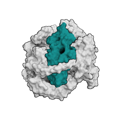
How to use information about interactions in HADDOCK?
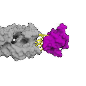
Docking with HADDOCK
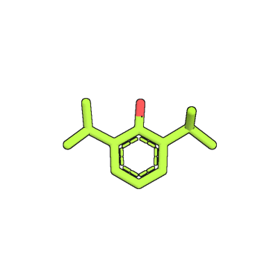
|

|
|
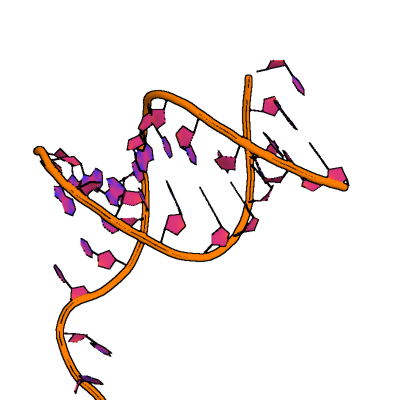
|
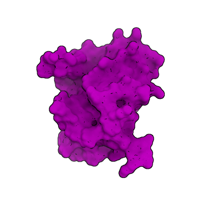
|
|
|
|
|||||
After docking: How to analyze docking results from HADDOCK or refine models?
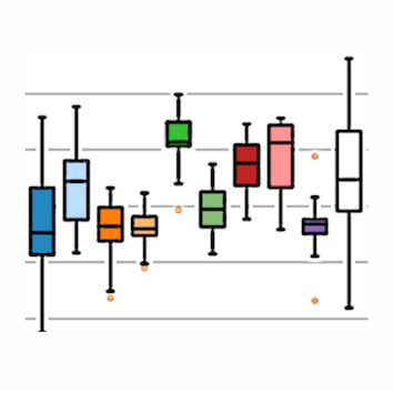
Structures
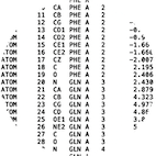
Best practice guide
The first step in your docking protocol is to know which molecules you want to find a complex for. This might sound easy, but it can be quite tricky. This section explains where to find or model input structures, how to edit them, and prepare them for HADDOCK.
Which structures are available?
Experimental structures
In the best-case scenario, there is an experimental structure available. All crystallographic, NMR, or cryo-EM structures protein structures are deposited in protein data banks:
-
Worldwide Protein Data Bank wwPDB
-
Protein Data Bank in Europe PDBe
-
The Research Collaboratory for Structural Bioinformatics Protein Data Bank RCSB PDB
-
Protein Data Bank Japan PDBj
-
Biological Magnetic Resonance Data Bank BMRB
Sequence and homologous proteins
In case when there is no experimental structure available for molecules of proteins of interest, one can use protein homologs as templates for protein modeling. There are multiple tools that help us to do so. Some online tools for homolog search are here:
Once one finds the protein homologs, some freely available software for homology model building are here:
-
- this online tool can both look for homologous proteins and build a protein model
-
- online version ModLoop for loop modeling
- local version for homology or comparative modeling of protein three-dimensional structures
Homology modeling using these tools is described in our tutorial here:
AI-generated structures
Using AI tools to generate structures is now becoming the standard. Nevertheless, one should always be careful when using it, as artifacts can be generated. Indeed, sterical clashes can be present. Also, long disordered regions with low predicted pLDDT around the protein will not help during the docking, as it may prevent the interaction of the structured domain. To prevent this, try to energy minimize the structure and remove spaghetti around the domain of interest.
- AlphaFoldDB: Hosted by the EBI/EMBL, it contains more than 2 milions predicted monomeric strucutre for a bunch of taxonomic spieces, that can be downloaded.
- UniProt: The UniProtKB now also provides, in the 'Structure' section, direct links to AlphaFoldDB, when available.
- Online ColabFold: Written and maintained by Sergey Ovchinnikov & Martin Steinegger, allows to run AlphaFold2 on a jupyter notebook using online resources.
- Local ColabFold: The GitHub repository of ColabFold host multiple solutions to install AlphaFold2 locally.
Modelling of peptides and mutations in proteins
- Point-mutations in HADDOCK are handled by changing the amino acid name and HADDOCK will fill the missing side chain atoms. This step is further described here and can be done using the pdb_mutate.py tool in haddock-tools.
Note that pdb_mutate.py will not create the new side-chain atoms (this is handled by HADDOCK). But if you prefer to have control of the side-chain conformation rather use tools like Pymol to introduce the mutation. This is even recommended in the case of a mutation to Histidine as the server can not automatically guess the protonation state if the side-chain is missing.
-
Pymol is an almost irreplaceable tool in the every-day life of a computational chemist. Pymol is often used in a number of HADDOCK tutorials for structure preparations as well as analysis of docking results.
- Pymol offers a lot of handy plugins that extend its usability, for example, peptide-building ,some of them can be found here:
- Pymol offers an option to mutate residues and choose the side chain conformation manually.
- Modelling of peptides using Pymol modeling scripts is described here.
-
- Rosetta, as well as plenty of other online tools have now functionalities with which you can build peptides from their sequences.
-
A list of modified amino acids supported by HADDOCK can be found here.
Modeling of small molecules
-
- OMEGA uses the SMILES strings as input to generate three-dimensional (3D) conformations of ligands. OMEGA was used by our group in previous rounds of the D3R challenge.
- license necessary
-
- open source chemoinformatics and machine learning software
-
- open source chemoinformatics software, with an online version accessible here.

-
to prepare topology and parameter files for the ligand in CNS format one can use:
-
ccp4-prodrg:
ccp4-prodrg -
the Automated Topology Builder (ATB) and Repository developed in the group of Prof. Alan Mark at the University of Queensland in Brisbane: https://atb.uq.edu.au/
-
BioBB using acpype: The BioExcel BioBuildingBlock (BioBB) library is hosting several tutorials on how to perform computations with a variety of different tools. Here is a link to the workflow used to parametrize ligands: https://mmb.irbbarcelona.org/biobb/workflows/tutorials/biobb_wf_ligand_parameterization.
-
The preparation of small molecules for docking is further described in the frequently asked questions page.
Using Molecular Dynamics for generating multiple conformations
Proteins are not rock-solid and HADDOCK can handle flexibility of the interface to a certain extent. Ensemble docking of conformations generated by molecular dynamics (MD) is an elegant way to account for larger conformational changes. There are a number of MD engines available for generating of conformations such as:
-
OpenMM: Can also be used within haddock3 itself as it is now a module (see refenement module / openmm)
Examples of using MD for HADDOCK are shown here:
Editing pdb files
Upon acquiring the input structures provided you might want to modify in one way or the other. This might not be very straightforward since pdb files have to meet strict formatting requirements and are rather lengthy to edit manually. The HADDOCK group has therefore developed a pipeline called PDB-Tools where pdb files can be submitted and edited it as needed. PDB-tools are available here:
- In your haddock3 environement: command line interface
- PDB-Tools Web: online version
- Local version of PDB-Tools: for a separated local installation
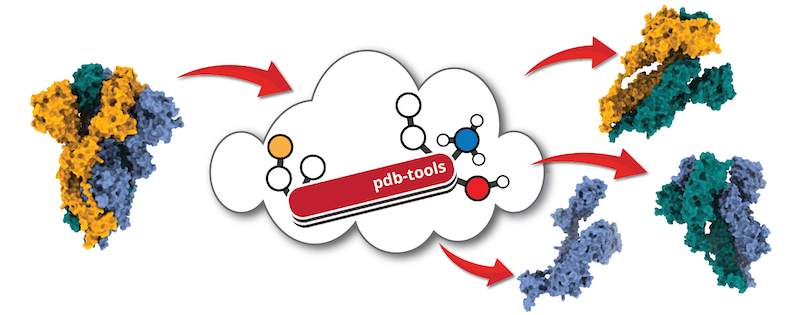
Tutorials:
Getting structures HADDOCK-ready
-
Preparation of coarse-grained pdb files
- HADDOCK can now handle large complexes containing up to 20 chains. An elegant way to increase the speed of these calculations is to use coarse graining with Martini.
-
Preparation of pdb files for the local version of HADDOCK2.4
-
Haddock tools are a bunch of useful tools available on [Github](https://github.com/haddocking/haddock-tools for use with local version of HADDOCK) that can be used to modify pdb or restraint files.
-
A list of modified amino acids and other molecule types supported by HADDOCK can be found here.
Dos and Don'ts
| Don't | Do instead |
|---|---|
| input a pdb file without checking it first | carefully inspect your pdb and remove any unwanted atoms (water molecules, ions, crystallization agents) |
| edit pdb files in Word, OpenOffice or LibreOffice editor | edit pdb files in an ASCII text editor |
| use residues with multiple occupancies (e.g. 124A, 124B) | use pdb_selaltloc to choose only one residue occupancy |
| use residues with overlapping numbering | use pdb_reres to renumber residues |
| use atoms with identical atom names for the same residue | edit your molecule with an ASCII text editor to make all atom names unique or use pdb_uniqname from our PDB-tools |
| use a pdb file with incorrect formatting | pdb formatting is very strict, check your file with pdb_validate and reload and export the file in Pymol if necessary |
Once you have your structures HADDOCK-ready you can go to the next step and define restraints.
Any more questions about pdb preparation for HADDOCK?
Have a look at:
Restraints
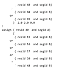
Best practice guide
As you probably saw in the previous step dedicated to structure preparation, there are many ways how to obtain structures of molecules that you want to dock. The next step is to define the way you expect these molecules to interact. HADDOCK is an information-driven tool, which means that the more available information about binding you have, the more meaningful your results will be. Based on the available information we distinguish between the following options:
- What information about binding is available?
- Complementary software related to restraints for HADDOCK
What information about binding is available?
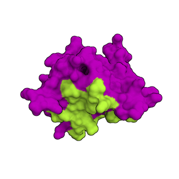
1. Information about the interface is available
Unambiguous Interaction restraints
If your predictions are highly reliable and you wish to have all of them applied during docking, define them as unambiguous restraints (using the unambig_fname parameter).
Unambiguous restraints are not subject to random removal, therefore all of them must be satisfied.
These can be for example:
- chain-break restraints generated by the
haddock3-restraint restrain_bodiescommand line - template-derived pairwise distance restraints (tutorial)
- MS crosslink data (tutorial)
- cryo-EM connectivity data (tutorial)
Ambiguous Interaction Restraints (AIRs)
Nevertheless, as in life, in science one also needs to be somewhat critical to the data one works with.
If you are not 100% sure about the interaction information and want to be cautious while incorporating it into your docking, use ambiguous interaction restraints (using the ambig_fname parameter).
Here, for each docking trial, a fraction of these restraints will be randomly removed, which ensures a wider sampling satisfying always a different subset of predefined restraints.
Thus, if some of the restraints are artificial, these can be filtered out if the complex satisfying them is unfavorable.
Of course, you can tune this random removal approach by modifying the npart parameter or turning it off by setting randremoval=false.
For AIRs, it is important to define the residues at the interface for each molecule based on experimental data that provides information on the interaction interface.
In the definition of those residues, one distinguishes between "active" and "passive" residues.
-
The "active" residues are of central importance for the interaction between the two molecules AND are solvent accessible. Either main chain or side chain relative accessibility should be typically > 40%, sometimes a lower cutoff might be used as well, for example, the HADDOCK server uses by default 15%. Throughout the simulation, these active residues are restrained to be part of the interface, if possible, otherwise incurring in a scoring penalty.
-
The "passive" residues are all solvent-accessible surface neighbors of active residues (<6.5Å). They contribute to the interaction but are deemed of less importance. If such a residue does not belong in the interface there is no scoring penalty.
In general, an AIR is defined as an ambiguous intermolecular distance between any atom of an active residue of molecule A and any atom of both active and passive residues of molecule B (and inversely for molecule B). This procedure can be performed:
- locally using the
haddock3-restraints active_passive_to_ambigcommand line - online using HADDOCK Restraints Generator web server
Using ambiguous restraints for docking is described in several tutorials:
Other kinds of restraints
-
Hydrogen bonds restraints: Another type of restraint not subject to random removal (accessed using
hbond_fnameparameter). -
DNA/RNA restraints: Automatically generated base-pair restraints using the
dnarest = trueparameter.
HADDOCK can utilize plenty of experimental information. Here we describe other types of restraints supported by HADDOCK:
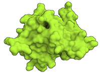
2. Information about the interface is not available
If there is no direct information about the interacting residues available, one can still browse through the available literature or employ bioinformatic prediction tools to gain some information about the potential complex. HADDOCK offers a plethora of ways for these scenarios.
Information about the quaternary structure of proteins (symmetry)
Symmetry restraints
HADDOCK offers the possibility to define multiple symmetry relationships within or in between molecules. This is done by using symmetry distance restraints. By defining multiple pairs of distances between the CA atoms of two chains, various symmetries can be enforced. Symmetry restraints are described in the manual here.
Ab-initio multi-body docking with symmetry restraints is described this Ab-initio tutorial (HADDOCK2.4).
Non-crystallographic symmetry restraints (NCS)
The NCS option imposes non-crystallographic symmetry restraints: It enforces that two molecules, a fraction thereof or even two sub-domains within the same molecule, should be identical without defining any symmetry operation between them. Non-crystallographic symmetry restraints are described in the manual here.
Ab-initio multi-body docking with NCS restraints is described here.
Membrane Z-positioning restraints
These restraints do not deal with symmetry, but can be useful in guiding the docking of membrane proteins. This type of restraint is used to keep segments within or outside of a defined Z-coordinate range. They can be used for docking of membrane proteins but can be used generically as well.
They are described in the HADDOCK manual here.
Ab-initio docking
Random interaction restraints
Haddock3 [rigidbody] module offers to define random AIRs from solvent-accessible residues (>20% relative accessibility) in case there is no experimental information, by turning on the ranair = true parameter.
The sampling will be done from the defined segments.
This can be useful for ab-initio docking to sample the entire protein surface.
To ensure a thorough sampling of the surface, the number of structures generated at the rigid-body stage [rigidbody] should be increased (e.g. sampling=10000), depending on the extent of the surface to be sampled.
These random restraints are described here.
Random interaction restraints are used in the binding site tutorial.
Center of mass restraints
Center of mass (COM) restraints are distance restraints that ensure close proximity of two molecules. Such restraints can be useful in multi-body (N>2) docking to ensure that all molecules are in contact and thus promote compactness of the docking solutions. Similarly to the contact surface restraints, they can be useful in combination with random interaction restraints definition (see above) or in the refinement of molecular complexes.
COM restraints are mentioned in multiple tutorials, for example:
- Refining the interface of the cryo-EM fitted models with HADDOCK
- HADDOCK 2.4 CASP-CAPRI T70 Ab-initio docking tutorial
- Modelling a homo-oligomeric complex from MS cross-links.
Surface contact restraints
Surface contact restraints can be useful in multi-body (N>2) docking to ensure that all molecules are in contact and thus promote compactness of the docking solutions.
As for the random AIRs, surface contact restraints can be used in ab-initio docking; in such a case it is important to have enough sampling of the random starting orientations and this significantly increases the number of structures for rigid-body docking.
They can be useful in combination with random interaction restraints definition (see above) or in the refinement of molecular complexes.
They can be turned on by setting the contact_airs = true parameter.
Optimal settings for docking using bioinformatics predictions
When we are less certain about the interacting residues, it is better to enhance sampling by increasing the number of structures generated in each phase of docking.
This can be performed by tuning:
- Increasing the number of generated complexes by tuning the
samplingparameter in[rigidbody]module. - Selecting more complexes to be refined:
select = 400parameter in[seletop]module. - Split the predicted AIRs into smaller subsets, and generate a
.tgzarchive.
| Parameter | Module/parameter | default value | optimal value |
|---|---|---|---|
Number of generated structures for rigid body docking [rigidbody] | | 1000 | 10000 |
| Provide multiple AIRs as tar gz archive | | .tbl | .tbl.gz |
| Number of trials for rigid body minimisation | | 5 | 1 |
Number of structures selected for later refinements in [seletop] | | 200 | 400 |
IMPORTANT NOTE: Splitting your very ambiguous interaction restraints into multiple files can allow further de-noising (in addition to randremoval = true). This is performed by generating multiple restraints files, combining them in a single .tgz archive and finally using it from the ambig_fname parameter.
Have a look at the examples using multiple ambiguous restraints:
- In your haddock3 local installation:
examples/docking-multiple-ambig - Online
Here is an example:
# General parameters
#####################
# ...
# Workflow / Modules
#####################
# ...
[rigidbody]
sampling = 10000
ambig_fname = "noisy_ambigs.tbl.tgz"
[seletop]
select = 400
# ... refinements steps ...
More about optimal settings for different docking scenarios can be found here.
Getting restraints HADDOCK-ready
Several methods can allow you to generate restraints for haddock3:
- locally using the
haddock3-restraintscommand line interface: Holds multiple subcommands that should cover the majority of the usages. - online using GenTBL server
Dos and Don'ts
| Don't | Do instead |
|---|---|
| define the entire protein as active | define only key interacting residues as active, if they are not known, define the surface of one molecule as passive |
Complementary software related to restraints for HADDOCK
In BonvinLab, a number of complementary web servers have been developed to help users to reevaluate restraints.
ARCTIC-3D
ARCTIC-3D, standing for Automatic Retrieval and Clustering of Interfaces in Complexes, is a data mining algorithm that searches for experimental interfaces in the PDB and cluster interaction sites together. It is also able to directly generate AIRs for haddock3.
CPORT
CPORT is an algorithm for the prediction of protein-protein interface residues. It combines six interface prediction methods into a consensus predictor.
Tutorials using CPORT:
DISVIS
DISVIS visualizes and quantifies the information content of distance restraints between macromolecular complexes.
Tutorial describing DisVis:
- DisVis tutorial
- HADDOCK2.4 tutorial for the use of MS crosslinks
- Integrative modelling of the RNA polymerase III apo complex
Any more questions about restraints for HADDOCK?
Have a look at:
Small-molecules / Ligands
Best practice guide
It's possible to dock small molecules using HADDOCK, but for that topology and parameter files for the ligand should be provided in CNS format.
Several sources exist to find/generate such files:
-
BioBB using acpype: The BioExcel BioBuildingBlock (BioBB) library is hosting several tutorials on how to perform computations with a variety of different tools. Here is a link to the workflow used to parametrize ligands: https://mmb.irbbarcelona.org/biobb/workflows/tutorials/biobb_wf_ligand_parameterization
-
ccp4-prodrg:
ccp4-prodrg -
the PRODGR server maintained by Daan van Aalten at Dundee University. This server allows you to draw your molecule or paste coordinates and will return topologies and parameter files in various formats, including CNS. You should turn on the electrostatic to obtain partial charges.
-
the Automated Topology Builder (ATB) and Repository developed in Prof. Alan Mark's group at the University of Queensland in Brisbane: https://atb.uq.edu.au/
-
Using OpenBabel and acpype: A simple set of two commands can generate CNS ready topology and parameters using both OpenBabel and acpype.
# Install OpenBabel and acpype
pip install acpype==2023.10.27 openbabel-wheel==3.1.1.21
# First standardise and add hydrogens to your pdb file using OpenBabel
obabel -ipdb <input_file.pdb> -opdb -O ligand.pdb -h
# Use acpype to generate cns parameters and topology
acpype -i ligand.pdb -o cns -t -j -a ambe
A more detailed description is written in the protein-ligand docking example. To increase the chance of getting the right ligand conformation, one can perform ensemble docking. In this scenario, multiple conformations can be generated as described here.
Use of multiple ligands at once
When using multiple ligands at once in the same docking run, several steps must be considered:
-
Atom types and residue names should not overlap with each other (nor with already existing definitions)
-
Topologies of different ligands must be merged into a single file and used in the
ligand_param_fname. -
Parameters of different ligands must be merged into a single file and used in the
ligand_top_fname.
Tutorials
-
HADDOCK2.4 ligand binding site tutorial: A tutorial demonstrating the use of HADDOCK in ab-initio mode to screen for potential ligand binding sites. The information from the ab-initio run is then used to setup a binding pocket-targeted protein-ligand docking run. We use as an example the multidrug exporter AcrB.
-
Metadynamics: This tutorial highlights the benefits of enhanced sampling using metadynamics to improve the predictive power of molecular docking for protein-small molecule targets, in the case of binding sites undergoing conformational changes. For this, we will first generate an ensemble of conformers for the target protein using GROMACS and PLUMED, before proceeding with the docking using HADDOCK.
-
HADDOCK covalent binding: This tutorial demonstrates how to use HADDOCK for the prediction of the three dimensional structure of a covalently bound ligand onto a receptor.
Publications
-
A. Basciu, P.I. Koukos, G. Malloci, A.M.J.J. Bonvin and A.V. Vargiu. Coupling enhanced sampling of the apo‐receptor with template‐based ligand conformers selection: performance in pose prediction in the D3R Grand Challenge 4. J. Comp. Aid. Mol. Des. 34, 149-162 (2020). A preprint can be downloaded from here.
-
P.I. Koukos, L.C. Xue and A.M.J.J. Bonvin. Protein-ligand pose and affinity prediction. Lessons from D3R Grand Challenge 3. J. Comp. Aid. Mol. Des. 33, 83-91 (2019).
-
A. Vangone, J. Schaarschmidt, P. Koukos, C. Geng, N. Citro, M.E. Trellet, L.C. Xue and A.M.J.J. Bonvin. Large-scale prediction of binding affinity in protein-small ligand complexes: the PRODIGY-LIG web server. Bioinformatics, 35, 1585–1587 (2019).
-
Z. Kurkcuoglu, P.I. Koukos, N. Citro, M.E. Trellet, J.P.G.L.M. Rodrigues, I.S. Moreira, J. Roel-Touris, A.S.J. Melquiond, C. Geng, J. Schaarschmidt, L.C. Xue, A. Vangone and A.M.J.J. Bonvin. Performance of HADDOCK and a simple contact-based protein-ligand binding affinity predictor in the D3R Grand Challenge 2. J. Comp. Aid. Mol. Des. 32, 175-185 (2018).
Optimal settings for docking of small molecules
| Parameter | module / parameter | default value | optimal value |
|---|---|---|---|
| Clustering method | | ||
| Cutoff for clustering | clust_cutoff | 7.5 | 2.5 |
Constant dieletric constant in [rigidbody] | dielec | rdie | cdie |
Reduce VdW energy component in [rigidbody] | w_vdw | 0.01 | 0 |
Constant dieletric constant in [flexref] | dielec | rdie | cdie |
Epsilon constant for the electrostatic energy term in [flexref] | epsilon | 1.0 | 10.0 |
Number of MD steps for rigid body high temperature TAD in [flexref] | mdsteps_rigid | 500 | 0 |
Number of MD steps during first rigid body cooling stage in [flexref] | mdsteps_cool1 | 500 | 0 |
Initial temperature for second TAD cooling step with flexible side-chain at the interfacein [flexref] | mdsteps_cool2 | 1000 | 500 |
Initial temperature for third TAD cooling step with fully flexible interfacein [flexref] | mdsteps_cool3 | 1000 | 300 |
Increase electrostatics component in [emref] | w_elec | 0.2 | 0.1 |
More about optimal settings for different docking scenarios can be found here.
Any more questions about small molecule docking with HADDOCK?
Have a look at:
Glycans

Best practice guide
HADDOCK also supports the docking of several carbohydrates. A list of glycan residues supported by HADDOCK can be found here. This page consists of the following chapters:
Tutorials
- HADDOCK3 protein-glycan modeling and docking: This tutorial shows how to use HADDOCK3 to dock a glycan to a protein, provided that some information exists about the protein binding site.
Publications
- A. Ranaudo, M. Giulini, A. Pelissou Ayuso and A.M.J.J. Bonvin. Modelling Protein-Glycan Interactions with HADDOCK. J. Chem. Inf. Mod. 64, 7816–7825 (2024).
Optimal settings for docking of glycans
| Parameter | Module / parameter | default value | optimal value |
|---|---|---|---|
| Clustering method | | ||
Cutoff for clustering in [clustrmsd] | clust_cutoff | 7.5 | 2.5 |
More about optimal settings for different docking scenarios can be found here.
FAQ
Any more questions about glycan docking with HADDOCK? Have a look at:
Peptides

Best practice guide
HADDOCK supports the docking of peptides as well. Since the secondary structure of short peptides is not always well defined, it is safer to dock an ensemble of multiple conformations. Different ways of generating these conformations are described here. More documentation about peptide docking with HADDOCK is in the following sections:
Tutorials
- HADDOCKing of the p53 N-terminal peptide to MDM2: This tutorial introduces protein-peptide docking using the HADDOCK web server. It also introduces the CPORT web server for interface prediction, based on evolutionary conservation and other biophysical properties.
Publications
-
C. Geng, S. Narasimhan, J. P.G.L.M. Rodrigues and A.M.J.J. Bonvin. Information-driven, ensemble flexible peptide docking using HADDOCK. Methods in Molecular Biology: Modeling Peptide-Protein Interactions. Eds Ora Schueler-Furman and Nir London. Humana Press Inc. 1561, 109-138 (2017).
-
A.D. Spiliotopoulos, P.L. Kastritis, A.S.J. Melquiond, A.M.J.J. Bonvin, G. Musco, W. Rocchia and A. Spitaleri. dMM-PBSA: a new HADDOCK scoring function for protein-peptide docking. Frontiers in Molecular Biosciences, 3:46 doi:10.3389/fmolb.2016.00046 (2016).
-
E. Deplazes, J. Davies, A.M.J.J. Bonvin, G.F. King and A.E. Mark. On the Combination of Ambiguous and Unambiguous Data in the Restraint-driven Docking of Flexible Peptides with HADDOCK: The Binding of the Spider Toxin PcTx1 to the Acid Sensing Ion channel (ASIC)1a. J. Chem. Inf. and Model. 56, 127-138 (2016).
-
J.P.G.L.M. Rodrigues, A.S.J. Melquiond and A.M.J.J. Bonvin. Molecular Dynamics Characterization of the Conformational Landscape of Small Peptides: A series of hands-on collaborative practical sessions for undergraduate students. Biochemistry and Molecular Biology Education, 44, 160-167 (2016).
-
M. Trellet, A.S.J. Melquiond and A.M.J.J. Bonvin. Information-driven modelling of protein-peptide complexes. Methods in Molecular Biology. Ed. Peng Zhou. Humana Press Inc. 221-239 (2015)
-
M. Trellet, A.S.J. Melquiond and A.M.J.J. Bonvin. A Unified Conformational Selection and Induced Fit Approach to Protein-Peptide Docking PLoS ONE, 8(3) e58769 (2013).
Optimal settings for docking of peptides
| Parameter | run.cns name | default value | optimal value |
|---|---|---|---|
| Distance matrix calculation | [ilrmsdmatrix] | ||
| Clustering method | [clustrmsd] | ||
| Cutoff for clustering | clust_cutoff | 7.5 | 5 |
| Flexible refinement | [flexref] | ||
| Number of MD steps for rigid body high temperature TAD | mdsteps_rigid | 500 | 2000 |
| Number of MD steps during first rigid body cooling stage | mdsteps_cool1 | 500 | 2000 |
| Number of MD steps during second cooling stage with flexible side-chains at interface | mdsteps_cool2 | 500 | 4000 |
| Number of MD steps during third cooling stage with fully flexible interface | mdsteps_cool3 | 500 | 4000 |
More about optimal settings for different docking scenarios can be found here.
FAQ
Any more questions about peptide docking with HADDOCK?
Have a look at:
DNA and RNA
Best practice guide
HADDOCK supports the docking of nucleic acids, including both DNA and RNA. Currently, only canonical nucleic acid bases are supported. They are listed here.
DNA and RNA nucleotide naming convention
In HADDOCK, DNA and RNA bases must adhere to a strict naming convention to be correctly recognized and interpreted by CNS.
DNA nucleotides:
- Adenosine:
DA - Thymine:
DT - Cytosine:
DC - Guanine:
DG
Note that DNA nucleotides are denoted by two-letter codes, starting at position 18 in the PDB file.
RNA nucleotides:
- Adenosine:
A - Uracil:
U - Cytosine:
C - Guanine:
G
Note that RNA nucleotides are denoted by single-letter codes, starting at position 18 in the PDB file.
Any residue labeled simply as T will be ignored during docking.
If you notice missing thymine residues in your DNA after docking, it is likely that all DNA residues were labeled incorrectly - following the RNA naming convention instead.
This would result in the molecule being treated as RNA rather than DNA.
Publications
-
Z. Kurkcuoglu and A.M.J.J. Bonvin. Pre- and post-docking sampling of conformational changes using ClustENM and HADDOCK for protein-protein and protein-DNA systems. Proteins: Struc. Funct. & Bioinformatics, 88, 292-306 (2020).
-
R.V. Honorato, J. Roel-Touris and A.M.J.J. Bonvin. MARTINI-based protein-DNA coarse-grained HADDOCKing. Frontiers in Molecular Biosciences, 6, 102 (2019).
-
M. van Dijk, K. Visscher, P.L. Kastritis and A.M.J.J. Bonvin. Solvated protein-DNA docking using HADDOCK. J. Biomol. NMR, 56, 51-63 (2013).
-
M. van Dijk and A.M.J.J. Bonvin Pushing the limits of what is achievable in protein-DNA docking. Benchmarking HADDOCK's performance.Nucl. Acid Res., 38, 5634-5647 (2010).
-
M. van Dijk and A.M.J.J. Bonvin A protein-DNA docking benchmark. Nucl. Acids Res. (2008), 36, e88, doi: 10.1093/nar/gkn386.
-
M. van Dijk, A.D.J. van Dijk, V. Hsu, R. Boelens and A.M.J.J. Bonvin Information-driven Protein-DNA Docking using HADDOCK: it is a matter of flexibility. Nucl. Acids Res., 34 3317-3325 (2006).
Tutorials
- Haddock3 basic protein-DNA docking tutorial: This tutorial demonstrates the use of Haddock3 for predicting the structure of a protein-DNA complex in which two protein units bind to the double-stranded DNA in a symmetrical manner (reference structure 3CRO). In addition to provided ambiguous restraints used to drive the docking, symmetry restraints are also defined to enforce symmetrical binding to the protein. This tutorial is using a local version of Haddock3, and therefore requires the use of a terminal and some basic command line expertise.
Optimal settings for docking of nucleic acids
| Module | Parameter | default value | optimal value |
|---|---|---|---|
[rigidbody]: Epsilon constant for the electrostatic energy term | epsilon | 10.0 | 78.0 |
[rigidbody]: Turn off desolvation component term | w_desolv | 1.0 | 0 |
[rigidbody]: Constant dielectric constant | dielec | rdie | cdie |
[flexref]: Epsilon constant for the electrostatic energy term | epsilon | 10.0 | 78.0 |
[flexref]: Turn off desolvation component term | w_desolv | 1.0 | 0 |
[flexref]: Constant dielectric constant | dielec | rdie | cdie |
[flexref]: Turn on automatic DNA base-pair restraints | dnarest_on | false | true |
[flexref]: Reduce TAD factor | tadfactor | 8 | 4 |
[flexref]: Reduce start temperature in 3rd cooling phase | temp_cool3_init | 1000 | 300 |
More about optimal settings for different docking scenarios can be found here.
FAQ
Any more questions about nucleic acids docking with HADDOCK? Have a look at:
Proteins
Best practice guide
As the name HADDOCK (High Ambiguity Driven protein-protein DOCKing) suggests, HADDOCK was originally developed for docking of proteins. Nowadays HADDOCK belongs to the state-of-the-art software in the protein-protein docking field, thus protein-protein documentation is the most comprehensive one. You can read more about protein-protein docking in the following sections:
Tutorials
HADDOCK3 versions
You can find tutorial using HADDOCK3:
- Online, at https://www.bonvinlab.org/education/HADDOCK3/
- In this manual, at tutorials
HADDOCK2.4 versions
This section holds links to tutorials using the HADDOCK2.X software.
-
HADDOCK2.4 local installation tutorial: A tutorial demonstrating the installation and use of a local installation of HADDOCK2.4. It demonstrates various docking scenarios. You will need for this a valid license of HADDOCK2.4.
-
HADDOCK2.4 basic protein-protein docking tutorial: A tutorial demonstrating the use of the HADDOCK web server to model a protein-protein complex using interface information derived from NMR chemical shift perturbation data. This tutorial does not require any Linux expertise and only makes use of our web server and PyMol for visualization/analysis.
-
HADDOCK2.4 MS cross-links tutorial: A tutorial demonstrating the use of cross-linking data from mass spectrometry to guide the docking in HADDOCK. This tutorial builds on our DisVis tutorial and illustrates various scenarios of using cross-linking data in HADDOCK. This tutorial does not require any Linux expertise and only makes use of our web server and PyMol for visualization/analysis.
-
DISVIS/HADDOCK2.4 oligomer puzzle: In this tutorial, you will have to solve an oligomer puzzle, namely predicting the correct oligomeric state of a symmetrical homomer complex based on a few (artificial) cross-links. The tutorial does not require any Linux expertise and only makes use of the DISVIS and HADDOCK web servers and PyMol for visualization/analysis.
-
HADDOCK2.4 CA-CA restraints guided docking tutorial: A tutorial demonstrating a template-based approach to model protein-protein complexes. It combines the PS-HomPPI web server to find suitable templates and generate CA-CA distance restraints and HADDOCK for the CA-CA guided modeling. This tutorial does not require any Linux expertise and only makes use of the PS-HomPPI and HADDOCK web servers and PyMol for visualization/analysis.
-
HADDOCK2.4 ab-initio, multi-body symmetrical docking tutorial: A tutorial demonstrating multi-body docking with HADDOCK using its ab-initio mode with symmetry restraints. It is based on a former CASP-CAPRI target (T70).
-
HADDOCK2.4 antibody-antigen docking tutorial: This tutorial demonstrates the use of HADDOCK2.4 for predicting the structure of an antibody-antigen complex using information about the hypervariable loops of the antibody and either the entire surface of the antigen or a loose definition of the epitope. This tutorial does not require any Linux expertise and only makes use of our web servers and PyMol for visualization/analysis.
Publications
-
A.M.J.J. Bonvin, E. Karaca, P.L. Kastritis & J.P.G.L.M. Rodrigues. Correspondence: Defining distance restraints in HADDOCK. Nature Protocols 13, 1503 (2018). Free online only access
-
A.M.J.J. Bonvin, C. Geng, M. van Dijk, E. Karaca, P. L. Kastritis, P.I. Koukos, Z. Kurkcuoglu, A.S.J. Melquiond, J.P.G.L.M. Rodrigues, J. Schaarschmidt, C. Schmitz, J. Roel-Touris, M.E. Trellet, S. de Vries, A. Vangone, L. Xue, G.C.P. van Zundert HADDOCK. In Encyclopedia of Biophysics, In press (2018).
-
G.C.P van Zundert, J.P.G.L.M. Rodrigues, M. Trellet, C. Schmitz, P.L. Kastritis, E. Karaca, A.S.J. Melquiond, M. van Dijk, S.J. de Vries and A.M.J.J. Bonvin. The HADDOCK2.2 webserver: User-friendly integrative modeling of biomolecular complexes. J. Mol. Biol., 428, 720-725 (2016).
-
G.C.P. van Zundert, A.S.J. Melquiond and A.M.J.J. Bonvin. Integrative modeling of biomolecular complexes: HADDOCKing with Cryo-EM data. Structure. 23, 949-960 (2015).
-
G.C.P. van Zundert, A.S.J. Melquiond and A.M.J.J. Bonvin. Integrative modeling of biomolecular complexes: HADDOCKing with Cryo-EM data. Structure. 23, 949-960 (2015).
-
J.P.G.L.M Rodrigues, E. Karaca and A.M.J.J. Bonvin. Information-driven structural modelling of protein-protein interactions. Methods in Molecular Biology: Molecular Modelling of Proteins. Ed. Andreas Kokul. Humana Press Inc. 399-424 (2015).
-
G.C.P. van Zundert and A.M.J.J. Bonvin. Modeling protein-protein complexes using the HADDOCK webserver. Methods in Molecular Biology: Protein Structure Prediction. Ed. Daisuke Kihara. Humana Press Inc., 163-179 (2014).
-
A.M.J.J. Bonvin, M. van Dijk, E. Karaca, P.L. Kastritis, A.S.J. Melquiond, C. Schmitz and S.J. de Vries HADDOCK In Encyclopedia of Biophysics, Ed. G.C.K. Roberts, Springer-Verlag Berlin Heidelberg (2013).
-
C. Schmitz, A.S.J. Melquiond, S.J. de Vries, E. Karaca, M. van Dijk, P.L. Kastritis and A.M.J.J. Bonvin Protein-protein docking with HADDOCK In: NMR in Mechanistic Systems Biology. Ed. I. Bertini, K.S. McGreevy and G. Parigi, Wiley-Blackwell, 512-535.
-
P.L. Kastritis, A.D.J. van Dijk and A.M.J.J. Bonvin Explicit Treatment of Water Molecules in Data-Driven Protein-Protein Docking: The Solvated HADDOCKing Approach Methods in Molecular Biology 819, Part 5, 355-374 (2012)
-
E. Karaca and A.M.J.J. Bonvin A multi-domain flexible docking approach to deal with large conformational changes in the modeling of biomolecular complexes. Structure, 19 555-565(2011).
-
P.L. Kastritis, I.H. Moal, H. Hwang, Z. Weng, P.A. Bates, A.M.J.J. Bonvin and J. Janin A structure-based benchmark for protein-protein binding affinity. Prot. Sci., 20, 482-41 (2011).
-
A.S.J. Melquiond and A.M.J.J. Bonvin Data-driven docking: using external information to spark the biomolecular rendez-vous. In: Protein-protein complexes: analysis, modelling and drug design. Edited by M. Zacharrias, Imperial College Press, 2010. p 183-209.
-
E. Karaca, A.S.J. Melquiond, S.J. de Vries, P.L. Kastritis and A.M.J.J. Bonvin Building macromolecular assemblies by information-driven docking: Introducing the HADDOCK multi-body docking server. Mol. Cell. Proteomics, 9, 1784-1794 (2010).
-
S.J. de Vries, M. van Dijk and A.M.J.J. Bonvin The HADDOCK web server for data-driven biomolecular docking. Nature Protocols, 5, 883-897 (2010).
-
S.J. de Vries, M. van Dijk and A.M.J.J. Bonvin The Prediction of Macromolecular Complexes by Docking. In: Prediction of Protein Structures, Functions, and Interactions (ed J. M. Bujnicki), John Wiley & Sons, Ltd, Chichester, UK (2009).
-
S. de Vries and A.M.J.J. Bonvin How proteins get in touch: Interface prediction in the study of biomolecular complexes. Curr. Pept. and Prot. Research, 9, 394-406 (2008).
-
A.D.J. van Dijk and A.M.J.J. Bonvin Solvated docking: introducing water into the modelling of biomolecular complexes.
-
S.J. de Vries and A.M.J.J. Bonvin Intramolecular surface contacts contain information about protein-protein interface regions. Bioinformatics, 22 2094-2098 (2006).
-
A.M.J.J. Bonvin Flexible protein-protein docking. Curr. Opin. Struct. Biol., 16, 194-200 (2006).
-
S.J. de Vries, A.D.J. van Dijk and A.M.J.J. Bonvin WHISCY: WHat Information does Surface Conservation Yield? Application to data-driven docking. Proteins: Struc. Funct. & Bioinformatics, 63, 479-489 (2006).
-
A.D.J. van Dijk, R. Boelens and A.M.J.J. Bonvin Data-driven docking for the study of biomolecular complexes. FEBS Journal, 272, 293-312 (2005).
-
C. Dominguez, R. Boelens and A.M.J.J. Bonvin HADDOCK: A protein-protein docking approach based on biochemical or biophysical information. J. Am. Chem. Soc., 125, 1731-1737 (2003).
Optimal settings
Default settings are optimal for protein-protein docking, however one can still modify parameters, such as the number of generated models.
More about optimal settings for different docking scenarios can be found here.
FAQ
A special section about docking of mutations with HADDOCK is dedicated in the frequently asked questions page.
Any more questions about protein-protein docking with HADDOCK? Have a look at:
Clustering methods implemented in Haddock3
Clustering of conformations and complexes is a key step in most workflows, as it allows us to observe convergence, redundancies, or even remove noise from singletons. Yet, two clustering methods are available in Haddock3:
- Clustering by Root Mean Squared Deviation:
[clustrmsd] - Clustering by Fraction of Comon Contacts:
[clustfcc]
Also, have a look at
RMSD clustering
In Haddock3, RMSD clustering module [clustrmsd] must always be preceded by the building of the RMSD matrix.
Indeed, the modules take the resulting RMSD matrix as input to build the dendrogram and cluster it.
Two modules can compute the RMSD matrix:
[rmsdmatrix]: Calculates of the RMSD matrix between all the models generated in the previous step.[ilrmsdmatrix]: Calculates the Interface Ligand Root Mean Square Deviation (ILRMSD) matrix.
Those two modules must be followed by the [clustrmsd] module; otherwise, only the pair-wise RMSD matrix will be computed, and clustering will not be performed.
[rmsdmatrix] module
The [rmsdmatrix] module allows you to define a subset of residues used to perform both the structural alignment and the RMSD computation.
For this, you need to specify a list of residues for each chain, using the parameter resdic_*, where * is the chainID.
As an example, to perform the selection of residues 12, 13, 14 and 15 from chain A and 1, 2, 3 from chain B, refine the following parameters:
[rmsdmatrix]
resdic_A = [12, 13, 14, 15]
resdic_B = [1, 2, 3]
This will result in the selection of those 7 residues to perform the structural alignment onto the reference and then compute the RMSD.
Full documentation about [rmsdmatrix] module is accessible here.
[ilrmsdmatrix] module
For the [ilrmsdmatrix] module, a different approach is taken.
Two parameters must be defined
receptor_chain: defining the chainID of the receptor. By default "A".ligand_chains: a list of other chain IDs that should represent the "ligands". If not set, all the remaining chains will be considered as ligand.
During the computational workflow, first, all the residue-residue contacts between the receptor and ligand are selected. This selection is then used to perform later structural alignment and RMSD computation.
Full documentation about [ilrmsdmatrix] module is accessible here.
[clustrmsd] module
Once the matrix has been computed, the clustering can be performed using the [clustrmsd] module.
The clustering is performed by first building a dendrogram, and then pruning the tree given two methods, accessible using the criterion parameter:
criterion = "maxclust": Pruning the tree to provide a defined number of clusters.criterion = "distance": Pruning the tree so members of the same cluster will share an RMSD distance between themselves inferior to the one defined.
When setting the criterion to "maxclust", the parameter n_clusters will be used to allow the definition of how many clusters you want.
While tuning the criterion to "distance", the parameter clust_cutoff will be used to set the threshold where to prune the tree. By doing so, you do not yet know how many clusters you will get in the end.
Remember that as this relies on manipulating the dendrogram, the way it is built will influence the results.
You can tune the linkage using the linkage parameter.
Full documentation about [clustrmsd] module is accessible here.
FCC clustering
Clustering by Fraction of Comon Contacts does not rely on rotation and translations but simply on the analysis of contacts. This is therefore much faster.
Full documentation about [clustfcc] module is accessible here.
Shared clustering parameters
Various parameters are shared between [clustrmsd] and [clustfcc] modules:
min_population: Threshold value employed to exclude clusters with less than this number of members. By default is 4.plot_matrix: Generates a plot displaying the matrix and the clustered members forwarded to the next step. By default is false.
Selecting cluster members
The module [seletopcluts] can be used to select clusters and their members.
Therefore, this module should be used after a clustering step (either [clustrmsd] or [clustfcc]).
This module holds three parameters:
top_clusters: how many clusters should be selectedtop_models: how many models in each selected cluster must be forwarded to the next stepsortby: How to sort clusters, by HADDOCK score or cluster size
Full documentation about [seletopcluts] module is accessible here.
Dos and Don'ts
| Don't | Do instead |
|---|---|
| set a too-loose or too-strict clustering cutoff | choose the right clustering cutoff for your system, help yourself by plotting the matrix |
| blindy accept the results of your clustering | if too many structures were left unclusters and you have few clusters, lower the clustering cutoff distance and/or the min_population parameters |
| take blindly the first ranked model/cluster | consider/examine multiple models/clusters, especially if they overlap within standard deviations in their score |
| consider the size of the cluster as an indication of its quality | use the cluster score and not its size for selecting best solutions (of course it is nice if the largest cluster is also the best scoring one) |
| consider/look only at the best model of a cluster | within one cluster, do visualize and compare several models (e.g. the top4) to get an idea of the precision and make sure the clustering worked properly |
| use RMSD matrix and clustering on >5000 models | use [clustfcc] instead |
Any more questions about clustering in Haddock3?
Have a look at:
Comparing your docking results to a known reference structure
The comparison to a reference structure has been streamlined, and can now be made simply by using the [caprieval] module.
This module will compute CAPRI criteria, of all the generated structures with respect to a reference one, with ligand-RMSD (l-RMSD), interface-ligand-RMSD (il-RMSD), Fraction of Native contacts (Fnat), DockQ and global-RMSD (RMSD) metrics.
This is also extended to the cluster level, enabling to rank clusters.
See here the full documentation related to the [caprieval] module.
Here is a schematic example of how to use the [caprieval] module:
# Some previous modules in the workflow
# ...

# Use CAPRIeval to compare previously generated models to a reference
[caprieval]
reference_fname = "target_complex.pdb"

# Some more modules until the end of the workflow
# ...
Notes:
- The best scoring complex will be used as a reference if the
reference_fnamein the[caprieval]module is not specified. - If a clustering step is placed before the
[caprieval]module, the analysis will also be extended to the cluster level, providing a more robust analysis.
Analysis command line interface
The haddock3-analyse command line generates interactive plots from the data obtained by a [caprieval] module directory.
Here is the documentation of the haddock3-analyse
Dos and Don'ts
| Don't | Do instead |
|---|---|
| take blindly the first ranked model/cluster | consider/examine multiple models/clusters, especially if they overlap within standard deviations in their score |
| consider the size of the cluster as an indication of its quality | use the cluster score and not its size for selecting the best solutions (of course it is nice if the largest cluster is also the best scoring one) |
| consider/look only at the best model of a cluster | within one cluster, do visualize and compare several models (e.g. the top4) to get an idea of the precision and make sure the clustering worked properly |
| take scores as proxies of binding affinity to compare different complexes | compare scores only within the same system/complex (i.e. to distinguish models for one docking run), or run [prodigy] module |
Any more questions about the analysis of the HADDOCK run?
Have a look at:
Haddock3 eco-system
Haddock3 can be used together with other tools that have been developed and maintained by the BonvinLab.
Local installation of tools
Here are some useful links to software that can be useful to solve your research question:
Featured research software
- pdb-tools: A dependency-free cross-platform swiss army knife for PDB files.
- prodigy: Predict the binding affinity of protein-protein and protein-ligand complexes from structural data
- arctic3d: Automatic Retrieval and ClusTering of Interfaces in Complexes from 3D structural information
- proABC-2: Deep learning framework to predict antibody paratope residues
- DisVis: Visualisation of conformational space restriction by distance restraints
- DeepRank-GNN-ESM: Deep learning framework for scroing protein-protein interaction docking poses.
Useful utilities
- haddock-restraints: Generate distance restraints to be used in HADDOCK
- haddock-runner: Run large scale HADDOCK simulations using multiple input molecules in different scenarios
- haddock-tools: Set of useful utility scripts developed by the BonvinLab group members
- haddock-mmcif: Encode information from a HADDOCK run to a cif file to be deposited in PDB-Dev
Webservers
We also provide online resources to perform computations related to the tools we developed.
Access our web portal here: https://wenmr.science.uu.nl/.
Haddock3 Web-Application
Here is the GitHub repository of the haddock3 web applications.
Online lectures
Haddock3 source code
Haddock3 is an open source software, and its source code can be downloaded from our haddocking/haddock3 GitHub repository.
Haddock3 source code structure
haddock3
|-- src/haddock
|   |-- clis
|   |   `-- cli*.py
|   `-- core
|   |   `-- *.py
|   `-- gears
|   |   `-- *.py
|   `-- libs
|   |   `-- lib*.py
|   `-- modules
|       |-- topology
|       |-- sampling
|       |-- refinement
|       |-- scoring
|       `-- analysis
`-- tests
|   |-- test_*.py
|   `-- golden_data
|       |-- *.pdb
|       |-- *.tsv
|       |-- *.tbl
`-- integration_tests
|   |-- test_*.py
|   |-- golden_data
|       |-- *.pdb
|       |-- *.tsv
|       |-- *.tbl
`-- examples
 |-- docking-examples
 |-- worflow.cfg
 `-- data
 |-- structure*.pdb
 |-- airs.tbl
 `-- reference_structure.pdb
Modules structure
defaults.yaml
This file contains all the parameter names and their default values. It also explains:
- the
defaultvalue to be used if the parameter is not defined in the configuration file. - the
typeof value to expect: string, integer, float, boolean, list - the allowed value range:
choices,minchars / maxchars,min / max,precision(number of digits for floating points) - a description of the parameter: its
title, and alongandshortdescriptions. - a
group: used to group parameters together. - the
explevelexpertise level:easy,expert,guru,hidden
This file is also used to build the documentation and the web-app.
Notes on expertise level
Note the explevel attribute to each parameter, allowing us to display (or not), parameters depending on the expertise level of the user.
While this is not used for local installation of haddock3, it is used at the web-application level to hide too techincal parameters to beginers (with easy expertise level).
__init__.py
Holds the module execution machinery.
cns/ directory
Contains CNS scripts related to the module: *.cns
python3 scripts *.py
Holds the module classes, methods, and functions related to the logic for the computation.
Tests
Unity tests
All unity tests scripts are located in the tests/ directory.
Each script starts with a test_ prefix.
They are supposed to be executed by pytest.
Integration tests
All integration tests scripts are located in the integration_tests/ directory.
Each script starts with a test_ prefix.
They are supposed to be executed by pytest.
End-to-end tests
The end-to-end tests are also examples that we provide to the users, to guide and help them understand how to use a module.
They also consist of predefined docking scenarios.
End-to-end tests are located in the examples/ directory.
We run on a daily basis most of the tests configuration files *-test.cfg present, tracking potential errors, hens making sure that haddock3 is functional after a new update.
How to cite haddock3
Citing haddock3
Here is the list of research articles related to haddock3:
- Description of haddock3: Marco Giulini#, Victor Reys#, Joao M. C. Teixeira#, Brian Jimenez-Garcia#, Rodrigo V. Honorato#, Anna Kravchenko, Xiaotong Xu, Raphaelle Versini, Anna Engel, Stefan Verhoeven, Alexandre M.J.J. Bonvin, HADDOCK3: A modular and versatile platform for integrative modelling of biomolecular complexes BioRxiv
- Haddock3 web-application: (soon!)
- Benchmarks:
- Focused Antibody-Antigen docking: M. Giulini, C. Schneider, D. Cutting, N. Desai, C. Deane and A.M.J.J. Bonvin. Towards the accurate modelling of antibody-antigen complexes from sequence using machine learning and information-driven docking. Bioinformatics 40:btae583, p. 1-11 (2024). BioRxiv
- Glycan docking: A. Ranaudo, M. Giulini, A. Pelissou Ayuso and A.M.J.J. Bonvin. Modelling Protein-Glycan Interactions with HADDOCK. J. Chem. Inf. Mod. 64, 7816–7825 (2024).
Citing haddock3 source-code
The haddock3 source code can be cited, as the GitHub repository contains a CITATION.cff file.
For this, go to https://github.com/haddocking/haddock3 and click on the Cite this repository on the right (see image).
Publications related to HADDOCK
Here is shorten list of important publications describing HADDOCK related work:
- First publication: C. Dominguez, R. Boelens and A.M.J.J. Bonvin. HADDOCK: A protein-protein docking approach based on biochemical or biophysical information. J. Am. Chem. Soc., 125, 1731-1737 (2003).
- HADDOCK webserver: S.J. de Vries, M. van Dijk and A.M.J.J. Bonvin The HADDOCK web server for data-driven biomolecular docking. Nature Protocols, 5, 883-897 (2010).
- HADDOCK2.2 webserver: G.C.P van Zundert, J.P.G.L.M. Rodrigues, M. Trellet, C. Schmitz, P.L. Kastritis, E. Karaca, A.S.J. Melquiond, M. van Dijk, S.J. de Vries and A.M.J.J. Bonvin. The HADDOCK2.2 webserver: User-friendly integrative modeling of biomolecular complexes. J. Mol. Biol., 428, 720-725 (2016).
- HADDOCK2.4 webserver: R.V. Honorato, M.E. Trellet, B. Jiménez-García1, J.J. Schaarschmidt, M. Giulini, V. Reys, P.I. Koukos, J.P.G.L.M. Rodrigues, E. Karaca, G.C.P. van Zundert, J. Roel-Touris, C.W. van Noort, Z. Jandová, A.S.J. Melquiond and A.M.J.J. Bonvin. The HADDOCK2.4 web server: A leap forward in integrative modelling of biomolecular complexes. Nature Prot., Advanced Online Publication DOI: 10.1038/s41596-024-01011-0 (2024).
- How to generate restraints for HADDOCK: A.M.J.J. Bonvin, E. Karaca, P.L. Kastritis & J.P.G.L.M. Rodrigues. Correspondence: Defining distance restraints in HADDOCK. Nature Protocols 13, 1503 (2018). Free online only access
For the complete list, please refere to our online BonvinLab resource.
Fundings
The development of Haddock3 is made possible thanks to the financial support from Horizon 2020, projects BioExcel 823830 and 101093290, EGI-ACE 101017567, and from the Netherlands e-Science Center (027.020.G13), that provided and still provides substantial fundings for software development. This allows the HADDOCK team to ensure software quality, improvements, maintenance, and user support.
User driven developments
In Haddock3, not only do we try to provide a powerful docking tool that can handle a variety of biomolecular entities, but we are also developing new modules and functionalities based on user requests. On a yearly basis, we ask users to fill out a survey, allowing us to focus on several different directions to improve the tool and make it more suitable for the community. Feature requests can also be performed directly from our GitHub repository issues.
20 years of HADDOCK
Haddock3 is the newest version of HADDOCK, an original idea initially developed by Dominguez, C., Boelens, R. & Bonvin, A. M. J. J. in 2003. For more than 20 years now, HADDOCK has been improved, going from its first description to several milestones, namely Haddock2.2, Haddock2.4, and now Haddock3.
In November 2023, we celebrated the 20-year anniversary of HADDOCK, where most of the incredible scientists who contributed to its development attended.
We wish to thank all the students, PhD candidates, and postdoctoral researchers for each of their contributions to the tool, as they have allowed us to continuously develop new methods and improve HADDOCK functionalities over the years.